Collisions

Newton provides a GPU-accelerated collision detection system with:

• Full shape-pair coverage — every shape type collides with every other shape type (see Shape Compatibility).

• Mesh-mesh contacts via precomputed SDFs for O(1) distance queries on complex geometry.

• Hydroelastic contacts that sample contacts across the contact surface for improved fidelity in torsional friction and force distribution, especially in non-convex and manipulation scenarios.

• Drop-in replacement for MuJoCo’s contacts — use Newton’s pipeline with SolverMuJoCo for advanced contact models (see MuJoCo Warp Integration).

This page starts with a conceptual overview of how geometry representations and narrow phase algorithms combine, then covers each stage in detail.

Conceptual Overview

Newton’s collision pipeline runs in two stages: a broad phase that quickly eliminates shape pairs whose bounding boxes do not overlap, followed by a narrow phase that computes the actual contact geometry for surviving pairs.

The narrow phase algorithm used for a given pair depends on how the shapes are represented:

        ---
config:
  theme: forest
  themeVariables:
    lineColor: '#76b900'

---
flowchart LR
  BP["Broad Phase<br/>(AABB culling)"] --> Triage
  subgraph Triage ["Pair Triage"]
    G1["Convex / primitive<br/>pairs"]
    G2["Mesh pairs<br/>(BVH or SDF)"]
  end
  subgraph NP ["Narrow Phase"]
    A["MPR / GJK"]
    B["Distance queries<br/>+ contact reduction"]
    C["Hydroelastic<br/>+ contact reduction"]
  end
  G1 --> A --> Contacts
  G2 --> B --> Contacts
  G2 -.->|"both shapes<br/>hydroelastic"| C --> Contacts
    

Geometry representations

1. Convex hulls and primitives — sphere, box, capsule, cylinder, cone, ellipsoid, and convex mesh shapes expose canonical support functions. These feed directly into the MPR/GJK narrow phase which produces contact points without further reduction. See Narrow Phase Algorithms.

2. Live BVH queries — triangle meshes that do not have a precomputed SDF are queried through Warp’s BVH (Bounding Volume Hierarchy). This path computes on-the-fly distance queries and generates contacts with optional contact reduction. It works out of the box but can be slow for high-triangle-count meshes. Hydroelastic contacts are not available on this path. See Mesh Collision Handling.

3. Precomputed SDFs — calling mesh.build_sdf(...) on a mesh precomputes a signed distance field that provides O(1) distance lookups. Primitive shapes can also generate SDF grids via ShapeConfig SDF parameters (see Shape Configuration). This path supports both distance-query and hydroelastic contact generation (with contact reduction). Hydroelastic contacts require SDF on both shapes in a pair. See Mesh Collision Handling and Hydroelastic Contacts.

Note

Contact reduction applies to the SDF-based and hydroelastic paths where many raw contacts are generated from distance field queries. The direct MPR/GJK path for convex pairs produces a small number of contacts and does not require reduction. See Contact Reduction.

Tip

For scenes with expensive collision (SDF or hydroelastic), running collide once per frame instead of every substep can significantly improve performance. See Common Patterns for the different collision-frequency patterns.

Contact Geometry

The output of the narrow phase is a set of contacts: lightweight geometric descriptors that decouple the solver from the underlying shape complexity. A mesh may contain hundreds of thousands of triangles, but the collision pipeline distills the interaction into a manageable number of contacts that the solver can process efficiently.

Each contact carries the following geometric data:

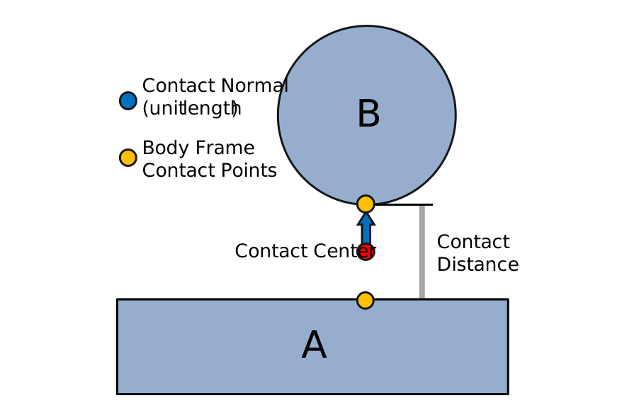
A contact between two shapes (A and B). The contact normal (blue, unit length) points from shape A to shape B. Body-frame contact points (yellow) are stored in each body’s local frame. The contact midpoint (red) — the average of the two world-space contact points — is not stored but is useful for visualization and debugging. The contact distance encodes the signed separation or penetration depth.

• Contact normal (world frame) — a unit vector pointing from shape A toward shape B.

• Contact points (body frame) — the contact location on each shape (rigid_contact_point0/1), stored in the parent body’s local coordinate frame.

• Contact distance — the signed separation between the two contact points along the normal. Negative values indicate penetration.

Because contacts are self-contained geometric objects, the solver never needs to query mesh triangles or SDF grids — it only works with the contact arrays stored in Contacts. See Contact Data for the full data layout.

MuJoCo Warp Integration

SolverMuJoCo (the MuJoCo Warp backend) ships with its own built-in collision pipeline that handles convex primitive contacts. For many use cases this is sufficient and requires no extra setup.

Newton’s collision pipeline can also replace MuJoCo’s contact generation, enabling SDF-based mesh-mesh contacts and hydroelastic contacts that MuJoCo’s built-in pipeline does not support.

Examples:

• Hydroelastic mesh contacts — newton/examples/contacts/example_nut_bolt_hydro.py

• SDF mesh contacts — newton/examples/contacts/example_nut_bolt_sdf.py

• Robot manipulation with SDF — newton/examples/contacts/example_brick_stacking.py

See Solver Integration for the full code pattern showing how to configure this.

Geometry-Pair Contact Behavior

The two tables below describe contacts generated by Newton’s CollisionPipeline only; they do not apply to contacts generated by the native MuJoCo CPU or MuJoCo Warp collision pipelines. The values are theoretical upper bounds per shape pair and collision pass before the shared rigid_contact_max capacity is applied. Actual counts vary with pose, margin, and collision settings.

CollisionPipeline primitive and convex-hull pairs

Shape A / Shape B	Plane	Sphere	Capsule	Ellipsoid	Cylinder	Box	Cone	Convex hull
Plane	5	1	2	1	4	4	5	5
Sphere	1	1	1	1	1	1	1	1
Capsule	2	1	2	1	5	5	5	5
Ellipsoid	1	1	1	1	1	1	1	1
Cylinder	4	1	5	1	5	5	5	5
Box	4	1	5	1	5	5	5	5
Cone	5	1	5	1	5	5	5	5
Convex hull	5	1	5	1	5	5	5	5

The plane–plane upper bound is five when at least one plane is finite. Two infinite planes produce no contacts.

CollisionPipeline mesh, heightfield, and SDF routes

V is a mesh vertex count, T_overlap is the number of overlapping triangles, and E is the number of collision edges. The estimated typical count is the sizing heuristic used for allocation, not a measured statistical average or a per-pair limit.

Pair or route	Reduced maximum (default)	Unreduced maximum	Estimated typical count	Notes
Triangle mesh–infinite plane	240	V_mesh	About 40	At most one candidate per mesh vertex.
Mesh/heightfield–sphere or ellipsoid	240	T_overlap	About 40	At most one contact per overlapping triangle.
Mesh/heightfield–other primitive or convex hull	240	5 * T_overlap	About 40	Each overlapping triangle uses the convex manifold path.
Mesh–mesh	240	E_A + E_B	About 40	Uses edge-vs-SDF queries, with BVH distance fallback when needed.
Heightfield–mesh	240	E_heightfield + E_mesh	About 40	Uses the mesh/SDF route with on-the-fly heightfield evaluation.
Hydroelastic SDF–SDF	240 by default	Geometry and buffer dependent	No fixed estimate	anchor_contact=True can add contacts beyond the reduced set.

The reduced maximum follows the current 240-slot contact-reduction layout. Disabling reduction exposes the geometry-dependent candidate bounds shown above.

Common pair guidance

Pair	Expected behavior	Backend notes	Asset guidance
Sphere–plane or sphere–box	A point contact.	Newton, MuJoCo Warp, and MuJoCo CPU use single-contact primitive paths.	Use one sphere unless the asset needs a finite support patch; then use multiple collision shapes or a surface-contact representation.
Capsule–plane or capsule–box	End-on contact is point-like; side-on contact can span the capsule axis.	Newton and both MuJoCo backends have multi-contact paths for the line-like side contact.	A single capsule is normally sufficient. Use a compound only when the physical profile is not capsule-shaped.
Box–plane or box–box	Face contact forms an area-supporting manifold; edge and corner contacts use fewer points.	Newton and both MuJoCo backends generate multi-point face contacts.	Prefer a single box for box-like parts; it is cheaper and usually more stable than a tessellated mesh.
Cylinder–box	A cylinder lying across a broad box face should have a manifold spanning its support region.	Newton generates a convex manifold. MuJoCo CPU can generate a multi-point manifold with multi-CCD enabled. MuJoCo Warp currently emits one contact for this pair even with enable_multiccd=True; contact location can alternate between the cylinder ends. This is a known discrepancy tracked in mujoco_warp#1555.	Keep a single cylinder with Newton contacts. While the MuJoCo Warp issue is open, use use_mujoco_contacts=False or, if that is not possible, approximate load-bearing regions with multiple collision shapes.

The MuJoCo Warp cylinder–box behavior above is a known discrepancy, not the intended single-contact behavior of the geometry pair. For non-convex assets, use a convex compound or Newton’s mesh/SDF paths rather than expecting one primitive to reproduce the surface. See Mesh Collision Handling and Simulation Tuning.

Collision Pipeline

Newton’s collision pipeline implementation supports multiple broad phase algorithms and advanced contact models (SDF-based, hydroelastic, cylinder/cone primitives). See Broad Phase and Shape Compatibility for details.

Basic usage:

# Create a pipeline with the desired broad phase mode
from newton import CollisionPipeline

pipeline = CollisionPipeline(
    model,
    broad_phase="sap",
)
contacts = pipeline.contacts()
pipeline.collide(state, contacts)

Quick Start

A minimal end-to-end example that creates shapes, runs collision detection, and steps the solver (see also the Introduction tutorial and example_basic_shapes.py — newton/examples/basic/example_basic_shapes.py):

import warp as wp
import newton

builder = newton.ModelBuilder()
builder.add_ground_plane()

# Dynamic sphere
body = builder.add_body(xform=wp.transform((0.0, 0.0, 2.0), wp.quat_identity()))
builder.add_shape_sphere(body, radius=0.5)

model = builder.finalize()
solver = newton.solvers.SolverXPBD(model, iterations=5)

state_0 = model.state()
state_1 = model.state()
control = model.control()
pipeline = newton.CollisionPipeline(model)
contacts = pipeline.contacts()

dt = 1.0 / 60.0 / 10.0
for frame in range(120):
    for substep in range(10):
        state_0.clear_forces()
        pipeline.collide(state_0, contacts)
        solver.step(state_0, state_1, control, contacts, dt)
        state_0, state_1 = state_1, state_0

Supported Shape Types

Newton supports the following geometry types via GeoType:

Type	Description
PLANE	Infinite plane (ground)
HFIELD	Heightfield terrain (2D elevation grid)
SPHERE	Sphere primitive
CAPSULE	Cylinder with hemispherical ends
BOX	Axis-aligned box
CYLINDER	Cylinder
CONE	Cone
ELLIPSOID	Ellipsoid
MESH	Triangle mesh (arbitrary, including non-convex; SolverMuJoCo collides its convex hull, see MuJoCo Solver)
CONVEX_MESH	Convex hull mesh

Note

SDF is collision data, not a standalone shape type. For mesh shapes, build and attach an SDF explicitly with mesh.build_sdf(...) and then pass that mesh to builder.add_shape_mesh(...). For primitive hydroelastic workflows, SDF generation uses ShapeConfig SDF parameters.

Shapes and Rigid Bodies

Collision shapes are attached to rigid bodies. Each shape has:

• Body index (shape_body): The rigid body this shape is attached to. Use body=-1 for static/world-fixed shapes.

• Local transform (shape_transform): Position and orientation relative to the body frame.

• Scale (shape_scale): 3D scale factors applied to the shape geometry.

• Margin (shape_margin): Surface offset that shifts where contact points are placed. See Margin and gap semantics.

• Gap (shape_gap): Extra detection distance that shifts when contacts are generated. See Margin and gap semantics.

• Source geometry (shape_source): Reference to the underlying geometry object (e.g., Mesh).

During collision detection, shapes are transformed to world space using their parent body’s pose:

# Shape world transform = body_pose * shape_local_transform
X_world_shape = body_q[shape_body] * shape_transform[shape_id]

Contacts are generated between shapes, not bodies. Depending on the type of solver, the motion of the bodies is affected by forces or constraints that resolve the penetrations between their attached shapes.

Collision Filtering

The collision pipeline uses filtering rules based on world indices and collision groups.

World Indices

World indices enable multi-world simulations, primarily for reinforcement learning, where objects belonging to different worlds coexist but do not interact through contacts:

• Index -1: Global entities that collide with all worlds (e.g., ground plane)

• Index 0, 1, 2, …: World-specific entities that only interact within their world

builder = newton.ModelBuilder()

# Global ground (default world -1, collides with all worlds)
builder.add_ground_plane()

# Robot template
robot_builder = newton.ModelBuilder()
body = robot_builder.add_link()
robot_builder.add_shape_sphere(body, radius=0.5)
joint = robot_builder.add_joint_free(body)
robot_builder.add_articulation([joint])

# Instantiate in separate worlds - robots won't collide with each other
builder.add_world(robot_builder)  # World 0
builder.add_world(robot_builder)  # World 1

model = builder.finalize()

For heterogeneous worlds, use begin_world() and end_world().

For large-scale parallel simulations (e.g., RL), replicate() stamps out many copies of a template environment builder into separate worlds in one call:

# Template environment: one sphere per world
env_builder = newton.ModelBuilder()
body = env_builder.add_body()
env_builder.add_shape_sphere(body, radius=0.5)

# Combined builder: global geometry + 1024 replicated worlds
main = newton.ModelBuilder()
main.add_ground_plane()  # global (world -1), shared across all worlds
main.replicate(env_builder, copy_count=1024)
model = main.finalize()

Note

MJWarp does not currently support heterogeneous environments (different models per world).

World indices are stored in shape_world, body_world, etc.

Collision Groups

Collision groups control which shapes collide within the same world:

• Group 0: Collisions disabled

• Positive groups (1, 2, …): Collide with same group or any negative group

• Negative groups (-1, -2, …): Collide with shapes in any positive or negative group, except shapes in the same negative group

Group A	Group B	Collide?	Reason
0	Any	❌	Group 0 disables collision
1	1	✅	Same positive group
1	2	❌	Different positive groups
1	-2	✅	Positive with any negative
-1	-1	❌	Same negative group
-1	-2	✅	Different negative groups

builder = newton.ModelBuilder()

# Group 1: only collides with group 1 and negative groups
body1 = builder.add_body()
builder.add_shape_sphere(body1, radius=0.5, cfg=builder.ShapeConfig(collision_group=1))

# Group -1: collides with everything (except other -1)
body2 = builder.add_body()
builder.add_shape_sphere(body2, radius=0.5, cfg=builder.ShapeConfig(collision_group=-1))

model = builder.finalize()

Self-collision within articulations

Self-collisions within an articulation can be enabled or disabled with enable_self_collisions when loading models. By default, adjacent body collisions (parent-child pairs connected by joints) are disabled via collision_filter_parent=True.

# Enable self-collisions when loading models
builder.add_usd("robot.usda", enable_self_collisions=True)
builder.add_mjcf("robot.xml", enable_self_collisions=True)

# Or control per-shape (also applies to max-coordinate jointed bodies)
cfg = builder.ShapeConfig(collision_group=-1, collision_filter_parent=False)

Controlling particle collisions

Use has_shape_collision and has_particle_collision for fine-grained control over what a shape collides with. Setting both to False is equivalent to collision_group=0.

builder = newton.ModelBuilder()

# Shape that only collides with particles (not other shapes)
cfg = builder.ShapeConfig(has_shape_collision=False, has_particle_collision=True)

# Shape that only collides with other shapes (not particles)
cfg = builder.ShapeConfig(has_shape_collision=True, has_particle_collision=False)

UsdPhysics Collision Filtering

Newton follows the UsdPhysics collision filtering specification, which provides two complementary mechanisms for controlling which shapes collide:

1. Collision Groups - Group-based filtering using UsdPhysicsCollisionGroup

2. Pairwise Filtering - Explicit shape pair exclusions using physics:filteredPairs

Collision Groups

In UsdPhysics, shapes can be assigned to collision groups defined by UsdPhysicsCollisionGroup prims. When importing USD files, Newton reads the collisionGroups attribute from each shape and maps each unique collision group name to a positive integer ID (starting from 1). Shapes in different collision groups will not collide with each other unless their groups are configured to interact.

# Define a collision group in USD
def "CollisionGroup_Robot" (
    prepend apiSchemas = ["PhysicsCollisionGroup"]
) {
}

# Assign shape to a collision group
def Sphere "RobotPart" (
    prepend apiSchemas = ["PhysicsCollisionAPI"]
) {
    rel physics:collisionGroup = </CollisionGroup_Robot>
}

When loading this USD, Newton automatically assigns each collision group a unique integer ID and sets the shape’s collision_group accordingly.

Pairwise Filtering

For fine-grained control, UsdPhysics supports explicit pair filtering via the physics:filteredPairs relationship. This allows excluding specific shape pairs from collision detection regardless of their collision groups.

# Exclude specific shape pairs in USD
def Sphere "ShapeA" (
    prepend apiSchemas = ["PhysicsCollisionAPI"]
) {
    rel physics:filteredPairs = [</ShapeB>]
}

Newton reads these relationships during USD import and converts them to shape_collision_filter_pairs.

Collision Enabled Flag

Shapes with physics:collisionEnabled=false are excluded from all collisions by adding filter pairs against all other shapes in the scene.

Shape Collision Filter Pairs

The shape_collision_filter_pairs list stores explicit shape pair exclusions. This is Newton’s internal representation for pairwise filtering (including pairs imported from UsdPhysics physics:filteredPairs relationships).

The built-in broad phases reject pairs of shapes attached to the same non-static body and static-static pairs. These inherent exclusions are therefore not stored in the explicit filter-pair list.

builder = newton.ModelBuilder()

# Add shapes
body_a = builder.add_body()
body_b = builder.add_body()
shape_a = builder.add_shape_sphere(body_a, radius=0.5)
shape_b = builder.add_shape_box(body_b, hx=0.5, hy=0.5, hz=0.5)

# Exclude this specific pair from collision detection
builder.add_shape_collision_filter_pair(shape_a, shape_b)

Filter pairs are automatically populated in several cases:

• Adjacent bodies: Parent-child body pairs connected by joints (when collision_filter_parent=True). For USD joints with two explicit bodies, physics:collisionEnabled controls this filter with inverse polarity; joints to world do not create a body-pair filter. Also applies to max-coordinate jointed bodies.

• Disabled self-collision: All shape pairs within an articulation when enable_self_collisions=False

• USD filtered pairs: Pairs defined by physics:filteredPairs relationships in USD files

• USD collision disabled: Shapes with physics:collisionEnabled=false (filtered against all other shapes)

The resulting filter pairs are stored in shape_collision_filter_pairs as a read-only set of (shape_index_a, shape_index_b) tuples (canonical order: a < b). Update shape_collision_filter_pairs before calling finalize() and rebuild the model to change collision filters.

USD Import Example

# Newton automatically imports UsdPhysics collision filtering
builder = newton.ModelBuilder()
builder.add_usd("scene.usda")

# Collision groups and filter pairs are now populated:
# - shape_collision_group: integer IDs mapped from UsdPhysicsCollisionGroup
# - shape_collision_filter_pairs: pairs from physics:filteredPairs relationships

model = builder.finalize()

Broad Phase and Shape Compatibility

CollisionPipeline provides configurable broad phase algorithms:

Mode	Description
NxN	All-pairs AABB broad phase. O(N²), suited to small worlds (<100 shapes per world).
SAP	Sweep-and-prune AABB broad phase. O(N log N), better for larger scenes with spatial coherence.
EXPLICIT	Uses precomputed shape pairs (default). Combines static pair efficiency with advanced contact algorithms.

ModelBuilder.finalize() computes Model.shape_contact_pair_count without enumerating pairs. The explicit pair array, Model.shape_contact_pairs, is constructed and cached on first access, normally when creating an explicit collision pipeline. SAP and NxN do not request this array. Hydroelastic setup uses the pipeline’s explicit pairs when supplied; otherwise, it constructs only its hydroelastic subset. Default pairs and counts use the collision topology captured during finalization; editing model arrays does not change them. Assigning None to model.shape_contact_pairs disables the model’s shape-contact pairs. When using the pair array directly in CUDA graph capture, access it once before capture to initialize its storage.

Explicit construction uses bounded temporary buffers and reuses equivalent worlds. Its final storage still scales with the number of compatible pairs, which can be quadratic in shapes per world. For large scenes, SAP avoids that array; its runtime candidate buffer is controlled separately by CollisionPipeline(shape_pairs_max=...). Choose that capacity to accommodate the scene’s overlapping candidates.

Explicit broad-phase setup warns when the configured list contains more than 100 million pairs and the busiest world contributes at least 20,000 pairs, including shared global pairs. These pairs are tested on every collision update; consider SAP for large worlds.

from newton import CollisionPipeline

# Default: EXPLICIT (precomputed pairs)
pipeline = CollisionPipeline(model)

# NxN for small scenes
pipeline = CollisionPipeline(model, broad_phase="nxn")

# SAP for larger scenes
pipeline = CollisionPipeline(model, broad_phase="sap")

contacts = pipeline.contacts()
pipeline.collide(state, contacts)

Shape Compatibility

Shape compatibility summary (rigid + soft particle-shape):

	Plane	HField	Sphere	Capsule	Box	Cylinder	Cone	Ellipsoid	ConvexHull	Mesh	SDF	Particle
Plane	[1]	[1]	✅	✅	✅	✅	✅	✅	✅	✅	✅	✅
HField	[1]	[1]	✅	✅	✅	✅	✅	✅	✅	✅⚠️	✅	✅
Sphere	✅	✅	✅	✅	✅	✅	✅	✅	✅	✅	✅	✅
Capsule	✅	✅	✅	✅	✅	✅	✅	✅	✅	✅	✅	✅
Box	✅	✅	✅	✅	✅	✅	✅	✅	✅	✅	✅	✅
Cylinder	✅	✅	✅	✅	✅	✅	✅	✅	✅	✅	✅	✅
Cone	✅	✅	✅	✅	✅	✅	✅	✅	✅	✅	✅	✅
Ellipsoid	✅	✅	✅	✅	✅	✅	✅	✅	✅	✅	✅	✅
ConvexHull	✅	✅	✅	✅	✅	✅	✅	✅	✅	✅	✅	✅
Mesh	✅	✅⚠️	✅	✅	✅	✅	✅	✅	✅	✅⚠️	✅⚠️	✅
SDF	✅	✅	✅	✅	✅	✅	✅	✅	✅	✅⚠️	✅	✅
Particle	✅	✅	✅	✅	✅	✅	✅	✅	✅	✅	✅	[2]

Legend: ⚠️ = Can be slow for meshes with high triangle counts; performance can often be improved by attaching a precomputed SDF to the mesh (mesh.build_sdf(...)).

[1] Plane and heightfield shapes are static (world-attached) in Newton; static-static pairs are filtered from rigid collision generation.

[2] Particle-particle interactions are handled by the particle/soft-body solver self-collision path, not by the shape compatibility pipeline in this table.

Note

Particle in this table refers to soft particle-shape contacts generated automatically by the collision pipeline. These contacts additionally require the shape to have particle collision enabled (ShapeFlags.COLLIDE_PARTICLES / ShapeConfig.has_particle_collision). For examples, see cloth and cable scenes that use the collision pipeline for particle-shape contacts.

Note

Heightfield representation: A heightfield (HFIELD) stores a regular 2D grid of elevation samples. For rigid contacts, Newton uses dedicated heightfield narrow-phase routes: heightfield-vs-convex uses per-cell triangle GJK/MPR, while mesh-vs-heightfield routes through the mesh/SDF path with on-the-fly triangle extraction from the grid. For soft contacts, the collision pipeline automatically samples the heightfield signed distance and normal.

Note

SDF in this table refers to shapes with precomputed SDF data. There is no GeoType.SDF enum value; this row is a conceptual collision mode for shapes carrying SDF resources. Mesh SDFs are attached through mesh.build_sdf(...) and provide O(1) distance queries.

Narrow Phase Algorithms

After broad phase identifies candidate pairs, the narrow phase generates contact points. The algorithm used depends on the shape types in each pair.

Convex Primitive Contacts

MPR (Minkowski Portal Refinement) and GJK

MPR is the primary algorithm for convex shape pairs. It uses support mapping functions to find the closest points between shapes via Minkowski difference sampling. Works with all convex primitives (sphere, box, capsule, cylinder, cone, ellipsoid) and convex meshes. Newton uses MPR for penetration depth computation (not EPA); GJK handles the separated-shapes distance query.

Multi-contact generation

For convex primitive pairs, multiple contact points are generated for stable stacking and resting contacts. The collision pipeline estimates buffer sizes based on the model; you can override this value with rigid_contact_max when instantiating the pipeline. The automatic capacity is a conservative heuristic based on colliding shape types, contact-pair metadata, and world layout. It generally grows linearly with replicated worlds, but it is not a guaranteed worst-case bound. When the estimate implies at least 256 MiB for the base rigid-contact buffers, the pipeline warns with the resolved capacity and the inputs that produced it. Pass an explicit rigid_contact_max to select the memory budget and silence the warning. Optional collision features and solvers may allocate additional per-contact memory.

Pipeline construction publishes the resolved rigid and soft capacities as model.rigid_contact_max and model.soft_contact_max, which later pipelines reuse as defaults; publish_capacity=False keeps a private pipeline’s capacities to itself. Before collision setup these are None; zero is a valid empty capacity. Contact-indexed Solver Observables are sized from the Contacts passed to solver.observables() instead.

Mesh Collision Handling

Mesh collisions use different strategies depending on the pair type:

Mesh vs Primitive (e.g., Sphere, Box)

Uses BVH (Bounding Volume Hierarchy) queries to find nearby triangles, then generates contacts between primitive vertices and triangle surfaces, plus triangle vertices against the primitive.

Important

Triangle winding order matters. Newton uses counter-clockwise (CCW) winding to determine the outward face normal of each triangle. The collision pipeline performs back-face culling: when a convex shape is on the back side of a triangle (behind the face normal), the contact is discarded. This prevents shapes that tunnel through a mesh surface from being trapped by inverted contact normals.

Supply mesh indices in CCW order when viewed from the outside of the surface. If your mesh has inconsistent or clockwise winding, convex shapes may pass through the surface without generating contacts.

Mesh vs Plane

Projects mesh vertices onto the plane and generates contacts for vertices below the plane surface.

Mesh vs Mesh

Two approaches available:

1. BVH-based (default when no SDF configured): Iterates mesh vertices against the other mesh’s BVH. Performance scales with triangle count - can be very slow for complex meshes.

2. SDF-based (recommended): Uses precomputed signed distance fields for fast queries. For mesh shapes, call mesh.build_sdf(...) once and reuse the mesh.

Warning

If SDF is not precomputed, mesh-mesh contacts fall back to on-the-fly BVH distance queries which are significantly slower. For production use with complex meshes, precompute and attach SDF data on meshes:

my_mesh.build_sdf(max_resolution=64)
builder.add_shape_mesh(body, mesh=my_mesh)

Tip

Build an SDF on every mesh that can collide, even when high-precision contacts are not required. A low-resolution SDF (e.g., max_resolution=64) uses very little memory yet still provides O(1) distance queries that are dramatically faster than the BVH fallback. Without an SDF, mesh-vs-mesh and mesh-vs-primitive contacts must walk the BVH for every query point, which dominates collision cost in most scenes. Attaching even a coarse SDF eliminates this bottleneck.

build_sdf() accepts several optional keyword arguments (defaults shown in parentheses):

mesh.build_sdf(
    max_resolution=256,                   # Max voxels along longest AABB axis; must be divisible by 8 (None)
    narrow_band_range=(-0.005, 0.005),    # SDF narrow band [m] ((-0.1, 0.1))
    margin=0.005,                         # Extra AABB padding [m] (0.05)
    shape_margin=0.001,                   # Shrink SDF surface inward [m] (0.0)
    scale=(1.0, 1.0, 1.0),                # Bake non-unit scale into the SDF (None)
    edge_lower_angle_threshold_rad=math.radians(0.1),  # Drop near-coplanar edges below this angle (0.1 deg)
    edge_concave_filter=True,             # Drop concave edges with two fully concave endpoints
    edge_box_absorption=False,            # Drop edges fully covered by another edge's oriented box
)

max_resolution sets the voxel count along the longest AABB axis (must be divisible by 8); voxel size is uniform across all axes. Use target_voxel_size instead to specify resolution in meters directly — it takes precedence over max_resolution when both are provided. Use narrow_band_range to limit the SDF computation to a thin shell around the surface (saves memory and build time). Set the SDF margin to at least the sum of the shape’s margin and gap so the SDF covers the full contact detection range. Pass scale when the shape will be added with non-unit scale to bake it into the SDF grid. shape_margin is mainly useful for hydroelastic collision where a compliant-layer offset is desired.

An SDF built without scale follows the shape’s current shape_scale. When every such shape has unit scale at construction, CollisionPipeline compiles its SDF queries for unit scale. To change shape_scale of such a shape afterwards, construct the pipeline with dynamic_shape_scale=True, which keeps the slower scaled queries. Otherwise, routing a rescaled shape whose queries were compiled for unit scale through mesh-SDF collision prints a device warning, and a later collide() call outside graph capture raises RuntimeError; graph replays alone do not raise. Mesh-plane and mesh-convex contacts read the current scale directly and do not trigger this diagnostic.

Changing shape_scale on mesh, convex-mesh, or heightfield shapes also requires updating shape_collision_radius, shape_collision_aabb_lower, and shape_collision_aabb_upper to match the new scale. The local collision bounds already include scale, and collision does not rescale them again; stale bounds can cause broadphase culling to omit candidate pairs. dynamic_shape_scale=True changes only unbaked texture-SDF queries and does not update these bounds or rebuild baked SDFs or heightfield collision data. To rebuild, recreate the affected shapes on a ModelBuilder with the new scale, then call finalize() and construct a new CollisionPipeline. For explicitly prebuilt mesh SDFs, first rerun build_sdf() with the new scale before adding the mesh to the builder.

Edge simplification. mesh.build_sdf(...) also runs a dihedral-angle pre-filter over the mesh’s manifold edges and caches the surviving subset on the mesh; the SDF-mesh contact pipeline picks up that cached set in preference to the unfiltered edges, which materially reduces edge-vs-shape work for typical CAD or scanned meshes. The default threshold (edge_lower_angle_threshold_rad=math.radians(0.1)) drops only edges that are geometrically coplanar to within 0.1 degrees, so it is safe for most meshes; raise it to prune more aggressively, set it to 0 to keep every manifold edge, or pass a negative value (e.g. -1.0) to opt out of the simplification pass entirely. By default, edge_concave_filter=True also drops a concave manifold edge when both endpoints are fully concave: every neighbor in each endpoint’s closed manifold one-ring lies on or outward from its angle-weighted tangent plane, with at least one neighbor strictly outward. The filter is skipped for sign_method="normal" because pseudo-normal SDFs do not define an unambiguous solid interior. Set edge_box_absorption=True to additionally drop manifold edges that are fully covered by another nearby edge’s oriented box — useful for densely tessellated curved surfaces. edge_box_half_normal/edge_box_half_normal_rel and edge_box_half_lateral/edge_box_half_lateral_rel tune the box extents (absolute metres or fractions of the mesh AABB diagonal); see build_sdf() for full parameter docs.

On-disk SDF cache. Pass cache_dir to persist the cooked SDF and skip the cook on subsequent runs:

mesh.build_sdf(max_resolution=64, cache_dir="./sdf_cache")

Entries are content-addressed by mesh data and build parameters; changing any of them produces a fresh entry automatically. shape_margin is applied at sample time and is not part of the cache key. The on-disk format is internal and may change between Newton versions — caches are invalidated and re-cooked transparently.

Note

Watertight meshes are preferred. An SDF works best on a closed surface, so meshes whose every edge is shared by exactly two triangles give the most reliable inside/outside classification. Newton detects this automatically via is_watertight and switches to a faster parity-based construction path when it applies. Non-watertight meshes fall back to the slower winding-number path; SDFs on terrain meshes work too, but mind the resolution (terrains have large extents so surface features are easy to under-resolve) and expect noticeably longer construction times.

Mesh simplification for collision

For imported models (URDF, MJCF, USD) whose visual meshes are too detailed for efficient collision, approximate_meshes() replaces mesh collision shapes with convex hulls, bounding boxes, or convex decompositions:

builder.add_usd("robot.usda")

# Replace all collision meshes with convex hulls (default)
builder.approximate_meshes()

# Or target specific shapes and keep visual geometry
builder.approximate_meshes(
    method="convex_hull",
    shape_indices=non_finger_shapes,
    keep_visual_shapes=True,
)

Supported methods: "convex_hull" (default), "bounding_box", "bounding_sphere", "coacd" (convex decomposition), "vhacd".

CoACD and V-HACD decompositions support opt-in disk caching for reuse across builders and processes, including automatic approximation during USD import. Mesh decomposition caching is disabled by default. Enable it by setting a directory through newton.config before importing a scene:

import newton

newton.config.cache_dir_meshes = ".cache/convex"
builder = newton.ModelBuilder()
builder.add_usd("robot.usda")  # Uses this cache for authored convex decompositions.

# Disable mesh decomposition caching for subsequent calls and imports.
newton.config.cache_dir_meshes = None

Explicit cache_dir directories on approximate_meshes() override the global setting. Omitting the argument or passing None uses config.cache_dir_meshes at call time. Asset downloads are controlled independently by config.cache_dir_assets and remain cached by default in the Newton cache directory (NEWTON_CACHE_PATH or the platform’s user cache location). Setting that to None keeps each download in a fresh temporary directory until process exit. The asset cache environment default is read when Newton is imported. These settings do not affect Mesh.build_sdf(), which retains its explicit, opt-in cache.

Cache directories are created if needed. Entries include the source geometry, effective decomposition options (including the hull-vertex limit), backend versions, and cache format version in their keys. Shape scales, transforms, and materials are applied independently, so cached parts can be reused by differently configured shapes. Missing, corrupt, or incompatible entries are recomputed; cache I/O errors are logged without preventing approximation. Backend dependencies must still be installed. Failed decompositions and fallback hulls are not cached. Delete the directory to reclaim disk space. Other approximation methods ignore cache_dir.

Cache locations are runtime settings; they are not authored in USD.

Note

approximate_meshes() modifies the builder’s shape geometry in-place. By default (keep_visual_shapes=False), the original mesh is replaced for both collision and rendering. Pass keep_visual_shapes=True to preserve the original mesh as a visual-only shape alongside the simplified collision shape.

Contact Reduction

Contact reduction is enabled by default. For scenes with many mesh-mesh interactions that generate thousands of contacts, reduction selects a significantly smaller representative set that maintains stable contact behavior while improving solver performance.

How it works:

1. Contacts are binned by normal direction (polyhedron face directions)

2. Within each bin, contacts are scored by spatial distribution and penetration depth

3. Representative contacts are selected to preserve coverage and depth cues

To disable reduction, set reduce_contacts=False when creating the pipeline.

Body-pair contact reduction (opt-in):

Bodies built from many colliders (a foot made of several spheres or capsules, a hand of boxes) produce one manifold per shape pair, so a single physical patch can reach the solver as dozens of near-redundant contacts. Optional body-pair reduction reduces primitive and convex contacts per body pair in a group mode of the global contact reducer, before they are written. Enable it with body_pair_reduction:

import newton

builder = newton.ModelBuilder()
builder.add_ground_plane()
model = builder.finalize()

pipeline = newton.CollisionPipeline(
    model,
    body_pair_reduction=newton.CollisionPipeline.BodyPairReductionConfig(cell_size=0.25),
)
contacts = pipeline.contacts()

Contacts are grouped by body pair, material class, normal bin and spatial cell. Each group keeps one depth representative, up to six sampled footprint extremes over all its contacts and up to six more over its touching contacts only, so speculative contacts cannot displace the support polygon. Mesh and heightfield contacts keep their per-shape-pair reduction. Only the kept contacts are written, and if a group cannot be registered in the table, the frame keeps every primitive and convex contact. It is an approximation: support is sampled, not exact, and keeping rim points can strengthen torsional friction. Selection is memoryless, so on curved or mesh supports the kept set can change between steps.

Shapes on one body share a group only when their shape_material_* values and their per-shape custom attributes match; BodyPairReductionConfig.material_attributes narrows the attributes that count. Call refresh_body_pair_reduction_groups() after changing them at runtime.

Buffers from the pipeline’s contacts() are stamped rigid_contact_body_pair_reduced when the scene has primitive or convex contact pairs; a scene of only meshes and heightfields reduces nothing by body pair and keeps unstamped buffers. Only a pipeline that stamps its buffers collides into a stamped buffer, and a solver accepts one only if it declares supports_body_pair_reduced_contacts; the others raise in step(), also during CUDA graph capture. SolverSteel supports it, except with contact_compliance. Body-pair reduction doesn’t support contact_matching="sticky" or hydroelastic contacts. Keep it off when it doesn’t reduce the end-to-end step time. To check, compare the step time and rigid_contact_count with it on and off: a count that stays near its unreduced value means little was reduced, or the group table was too small and frames kept every contact (raise BodyPairReductionConfig.hashtable_size_factor).

This body-pair reduction API is experimental and may change without prior notice.

Configuring contact reduction (HydroelasticSDF.Config):

For hydroelastic and SDF-based contacts, use Config to tune reduction behavior:

from newton.geometry import HydroelasticSDF

config = HydroelasticSDF.Config(
    reduce_contacts=True,           # Enable contact reduction (default)
    buffer_fraction=0.2,            # Reduce GPU buffer allocations (default: 1.0)
    normal_matching=True,           # Align reduced normals with aggregate force
    anchor_contact=False,           # Optional center-of-pressure anchor contact
)

pipeline = CollisionPipeline(model, sdf_hydroelastic_config=config)

Other reduction options:

Parameter	Description
normal_matching	Rotates selected contact normals so their weighted sum aligns with the aggregate force direction from all unreduced contacts. Preserves net force direction after reduction. Default: True.
anchor_contact	Adds an anchor contact at the center of pressure for each normal bin to better preserve moments. Default: False.
margin_contact_area	Deprecated area used for speculative-contact activation stiffness. It remains effective during the deprecation period. Default: 0.01.

Shape Configuration

Shape collision behavior is controlled via ShapeConfig:

Collision control:

Parameter	Description
collision_group	Collision group ID. 0 disables collisions. Default: 1.
collision_filter_parent	Filter collisions with adjacent body (parent in articulation or connected via joint). Default: True.
has_shape_collision	Whether shape collides with other shapes. Default: True.
has_particle_collision	Whether shape collides with particles. Default: True.

Geometry parameters:

Parameter	Description
margin	Surface offset used by narrow phase. Pairwise effect is additive (m_a + m_b): contacts are evaluated against the signed distance to the margin-shifted surfaces, so resting separation is m_a + m_b. Helps thin shells/cloth stability and reduces self-intersections. Default: 0.0.
gap	Additional detection threshold. Pairwise effect is additive (g_a + g_b). Broad phase expands each shape AABB by (margin + gap) per shape; narrow phase then keeps a candidate contact when d <= g_a + g_b (with d measured relative to margin-shifted surfaces). Increasing gap detects contacts earlier and helps reduce tunneling. Default: None (uses builder.rigid_gap, which defaults to 0.1).
is_solid	Whether shape is solid or hollow. Affects inertia and SDF sign. Default: True.
is_hydroelastic	Whether the shape uses SDF-based hydroelastic contacts. Both shapes in a pair must have this enabled. See Hydroelastic Contacts. Default: False.
kh	Hydroelastic contact stiffness coefficient. Under the default linear pressure law, pressure scales with kh and penetration depth; contact force also scales with contact area. Default: 1.0e10.

Margin and gap semantics (where vs when):

• Where contacts are placed is controlled by margin.

• When contacts are generated is controlled by gap.

For a shape pair (a, b):

• Pair margin: m = margin_a + margin_b

• Pair gap: g = gap_a + gap_b

• Surface distance (true geometry, no offsets): s

• Contact-space distance used by Newton: d = s - m

Contacts are generated when:

\[d \leq g \quad\Leftrightarrow\quad s \leq (m + g)\]

Broad phase uses the same idea by expanding each shape AABB by:

\[margin_i + gap_i\]

This keeps broad-phase culling and narrow-phase contact generation consistent. The solver enforces d >= 0, so objects at rest settle with surfaces separated by margin_a + margin_b.

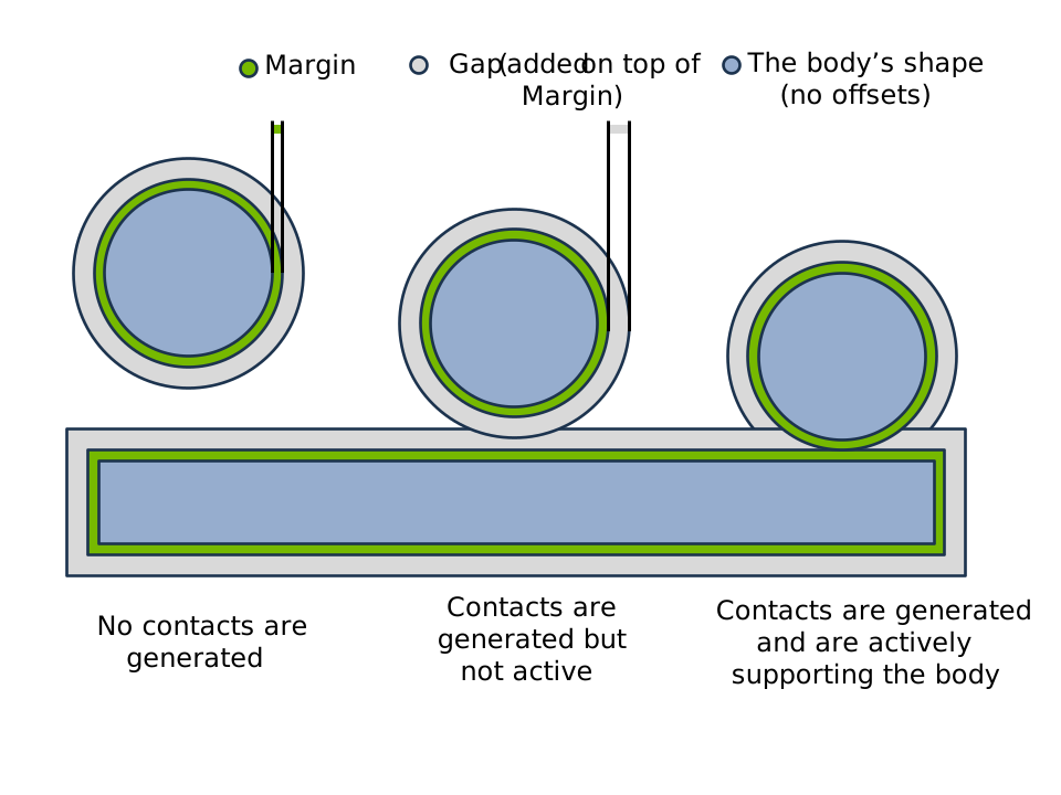
Margin sets contact location (surface offset), while gap adds an early detection distance on top of margin. Left: no contact generated. Middle: contact generated but not yet active. Right: active contact support.

SDF configuration (primitive generation defaults):

Parameter	Description
sdf_max_resolution	Maximum SDF grid dimension (must be divisible by 8) for primitive SDF generation.
sdf_target_voxel_size	Target voxel size for primitive SDF generation. Takes precedence over sdf_max_resolution.
sdf_narrow_band_range	SDF narrow band distance range (inner, outer). Default: (-0.1, 0.1).
sdf_padding	Primitive SDF AABB padding. For hydroelastic shapes this must cover margin + gap. When unset, Newton supplies that required padding.

For mesh-backed hydroelastic shapes, the padding passed to build_sdf() must likewise be at least margin + gap. Newton reports an actionable error when an attached SDF records smaller construction padding. When attaching externally precomputed texture data with create_from_data(), pass the original AABB padding through construction_padding. If that padding is unknown, shape validation rejects the SDF because Newton cannot verify that it covers the hydroelastic contact band.

The configure_sdf() helper sets SDF and hydroelastic options in one call:

builder = newton.ModelBuilder()
cfg = builder.ShapeConfig()
cfg.configure_sdf(max_resolution=64, is_hydroelastic=True, kh=1.0e11)

Example (mesh SDF workflow):

cfg = builder.ShapeConfig(
    collision_group=-1,           # Collide with everything
    margin=0.001,                 # 1mm margin
    gap=0.01,                     # 1cm detection gap
)
my_mesh.build_sdf(max_resolution=64)
builder.add_shape_mesh(body, mesh=my_mesh, cfg=cfg)

Builder default gap:

The builder’s rigid_gap (default 0.1) applies to shapes without explicit gap. Alternatively, use builder.default_shape_cfg.gap.

Speculative contacts (velocity-adapted gaps)

A fixed gap uses the same detection distance regardless of motion. Speculative contacts retain a separated rigid-contact candidate when its contact points can close the separation before the next collision update.

For a candidate with current contact-space separation d, authored pair gap g, normal-directed closing speed v, collision-update horizon dt, and configured limit e_max, the effective admission distance is:

\[g_{effective} = \max\left(g, \min\left(v\,dt, e_{max}\right)\right)\]

The contact is kept when d <= g_effective. Newton computes v from relative linear and angular velocity at the contact points. Common motion and receding motion therefore do not enlarge the gap. Broad phase uses a conservative motion bound; narrow phase applies the normal-directed test above.

The configured maximum extension is one limit for the shape pair, not a per-shape distance to add twice. If collision detection is skipped between solver substeps, sufficiently fast bodies can travel beyond that extension and tunnel through one another.

newton.CollisionSubstepScheduler reduces this risk by varying how often collision detection runs within a frame. The total number of simulation substeps remains fixed. The scheduler always runs collision detection at the beginning of a frame, tracks a conservative bound derived from the currently observed rigid-shape velocities on the device, and runs additional collision passes when that bound exhausts the available speculative distance or the previous collision prediction horizon expires, whichever occurs first. A drop in observed speed does not extend a previously selected horizon. The bound assumes that two bodies may move directly toward one another at the maximum observed shape speed:

states = (model.state(), model.state())
pipeline = newton.CollisionPipeline(
    model,
    speculative_contact_gap_max=0.1,
)
contacts = pipeline.contacts()

def collide(state, collision_dt):
    pipeline.collide(state, contacts, dt=collision_dt)

def substep(state_in, state_out, substep_dt):
    solver.step(state_in, state_out, control, contacts, substep_dt)

schedule = newton.CollisionSubstepScheduler(
    pipeline,
    states,
    collision_callback=collide,
    substep_callback=substep,
    frame_dt=1.0 / 60.0,
    substeps=10,
    collision_dt_max=1.0 / 120.0,
)
schedule.step()

During the collision callback, the scheduler’s pipeline retains candidates within a pairwise distance reserve of at least speculative_contact_gap_max, regardless of approach velocity. Authored gaps and physical margins are preserved. The callback must use the pipeline passed to the scheduler. Calls outside the callback retain velocity-adapted admission.

Gravity, slowing, and turning consume this reserve without unconditionally forcing a refresh. Refreshes occur when the travel estimate approaches the reserve or the previous horizon expires. The next-step estimate includes the speed increase observed over the preceding substep. This is not a bound on unobserved forces or impulses. Shapes with rigid collision disabled do not affect the schedule or overflow reporting. The final substep is checked for overflow.

The reserve may retain more contacts than velocity-adapted admission. Measure both total runtime and refresh counts, and size contact buffers accordingly. Fast motion can still require a refresh every substep.

The same step() call works directly or inside CUDA graph capture; callbacks must therefore be capture-safe and preallocate their storage. The scheduler always executes every configured solver substep. Its two states are ping-pong buffers, so the substep count must be even. schedule.interval_overflow is set when observed per-substep or accumulated travel exceeds the budget; in that case, increase the substep count or the speculative extension limit. Collision prediction horizons are capped at the next frame boundary, where contacts are always refreshed.

Set collision_dt_max to cap the time between collision passes independently of the travel estimate. For example, 1.0 / 120.0 requests collision detection at least 120 times per second. The scheduler rounds the interval down to a whole number of solver substeps and rejects a limit shorter than one substep. Intervals need not divide the frame’s substep count: with 14 substeps and a limit of six substeps, a stationary scene refreshes at substeps 0, 6, and 12, with the final horizon shortened to two substeps. Limits larger than frame_dt are capped at one frame.

CUDA graph capture records a conditional branch for each possible whole-substep horizon, up to the configured limit or the remaining frame duration. Supporting more horizons increases graph size and capture cost; a smaller collision_dt_max reduces the number of branches.

The scheduler is an experimental optimization for rigid contacts, not continuous collision detection. It does not support particles. It observes acceleration, impulses, and user-prescribed velocity changes only after a substep completes, so abrupt motion can still cross thin geometry within one substep. interval_overflow diagnoses limits implied by observed velocity; it cannot predict an acceleration that has not occurred yet. Choose the solver substep size for the expected acceleration and impulses.

Enable the feature with the keyword-only speculative_contact_gap_max constructor argument:

pipeline = newton.CollisionPipeline(
    model,
    speculative_contact_gap_max=0.1,
)

pipeline.collide(state, contacts, dt=1.0 / 60.0)

The per-call dt is the time [s] until the next planned CollisionPipeline.collide() call, including skipped solver substeps, and is required when speculative contacts are enabled. dt=0.0 uses only the authored gaps. speculative_contact_gap_max caps the velocity-derived detection gap [m]; it must be non-negative and finite. 0.0 does not enlarge authored gaps.

Speculation changes when a contact is retained, not its geometry: contact points remain at their current separation rather than a predicted impact pose. Mesh and SDF contact reduction preserves representative close-clearance and early-impact candidates.

Note

Speculative contacts are opt-in and currently apply to rigid, non-hydroelastic contacts. They do not compute a time of impact or advance bodies to impact.

Common Patterns

Creating static/ground geometry

Use body=-1 to attach shapes to the static world frame:

builder = newton.ModelBuilder()

# Static ground plane
builder.add_ground_plane()  # Convenience method

# Or manually create static shapes
builder.add_shape_plane(body=-1, xform=wp.transform_identity())
builder.add_shape_box(body=-1, hx=5.0, hy=5.0, hz=0.1)  # Static floor

Setting default shape configuration

Use builder.default_shape_cfg to set defaults for all shapes:

builder = newton.ModelBuilder()

# Set defaults before adding shapes
builder.default_shape_cfg.ke = 1.0e6
builder.default_shape_cfg.kd = 1000.0
builder.default_shape_cfg.mu = 0.5
builder.default_shape_cfg.is_hydroelastic = True
builder.default_shape_cfg.sdf_max_resolution = 64  # Primitive SDF defaults

Soft contacts (particle-shape)

Soft contacts are generated automatically when particles are present. They use a separate margin:

# Set the soft-contact detection gap (slack added to the particle radius)
pipeline = CollisionPipeline(model, soft_contact_gap=0.01)
contacts = pipeline.contacts()
pipeline.collide(state, contacts)

# Access soft contact data
n_soft = contacts.soft_contact_count.numpy()[0]
particles = contacts.soft_contact_particle.numpy()[:n_soft]
shapes = contacts.soft_contact_shape.numpy()[:n_soft]

With full-surface deformable-rigid mesh contacts enabled, detection retains the returned feature pairs, including endpoint contacts. SolverVBD selects force contributions inside each consuming kernel using its current particle and body positions, including during CUDA graph replay. Selection can change without another collision detection; it does not change the contact count, row order, or detected geometry. Coupling copies ownership and mesh provenance; the consuming solver evaluates eligibility. If the source contact buffer has overflowed, VBD bypasses geometric selection for stored mesh rows, including through coupling. A mesh row still needs a resolved inside/outside sign and at least one active soft participant to contribute forces. Rigid-soft division-plane constraints consume the detected rows independently of force selection.

Reverse rigid-vertex/soft-triangle contacts test the soft target’s neighbors and retain one eligible owner for a shared soft edge or vertex. They remain separate force contributions from soft-vertex/rigid-triangle queries. Full-surface mesh detection includes all rigid triangle edges, independently of SDF-selected edges. If the narrow vertex sign query fails, an expanded query supplies the sign for nearby vertex-triangle rows and, for an interior point, a recovery contact. Pairs whose sign remains unresolved are retained for DAT but do not contribute VBD forces until a subsequent detection resolves their sign. Edge penetration-recovery records are not ordinary edge-edge quadrature samples.

Full-surface mesh contact costs

Full-surface contact catches rigid features that can pass between deformable vertices, which is useful for coarse cloth. On finely tessellated or complex rigid meshes, however, retaining nearby feature pairs can produce many more records than particle-only contacts or SDF minimization. This increases contact storage and can substantially increase both collision detection and VBD solve time. Larger contact bands also admit more pairs. Profile the intended scene; the cost depends on mesh resolution, geometry, and contact density.

CollisionPipeline automatically estimates mesh contact storage. Set soft_contact_max to choose the total soft-contact capacity explicitly. The estimate is not an upper bound: dense patches can still overflow. The mesh overflow warning prints the current soft_contact_max and the required count for that collision pass. Increase soft_contact_max to at least that count, and verify that contacts fit throughout the simulation before relying on the results; later frames may require more storage.

This setting controls reserved storage, not the contact band or the number of feature pairs queried. Lowering capacity can save memory but produces incomplete contacts if it is too small; it is not a way to reduce query work while preserving the same contacts. The edge and vertex queries and the processing of their records remain a runtime cost even when the buffer is sized appropriately.

Collision frequency in the simulation loop

These patterns apply to contacts generated by CollisionPipeline; they do not control collision detection performed inside a solver. For example, SolverMuJoCo generates contacts internally when use_mujoco_contacts=True (see Collision pipeline), while SolverVBD handles particle self-contact internally according to the self-contact slot of collision_frequency / collision_frequency_type.

With rigid_soft_enable_dat=True, SolverVBD additionally truncates rigid pose and particle updates against the division planes of the rigid-soft contacts its owned CollisionPipeline reports, using the rigid entries of collision_frequency and collision_frequency_type as the detection cadence that anchors those planes. That slot may not be NONE while the option is enabled, and when particle self-contact truncation is also active the rigid and self-contact slots must share an equivalent schedule.

Start by calling collide every substep when debugging contact behavior. This keeps contacts current as bodies move. Once the behavior is acceptable, calling collide less often can reduce collision cost, especially for hydroelastic or SDF-heavy scenes.

These are the common loop patterns:

Every substep (the debugging baseline, used by most basic examples):

for frame in range(num_frames):
    for substep in range(sim_substeps):
        pipeline.collide(state_0, contacts)
        solver.step(state_0, state_1, control, contacts, dt=sim_dt)
        state_0, state_1 = state_1, state_0

Once per frame (faster, but contacts can become stale between substeps):

for frame in range(num_frames):
    pipeline.collide(state_0, contacts)
    for substep in range(sim_substeps):
        solver.step(state_0, state_1, control, contacts, dt=sim_dt)
        state_0, state_1 = state_1, state_0

Every N substeps trades contact freshness for collision cost. Use a positive integer: 1 means every substep, while values greater than or equal to sim_substeps reduce this frame-local loop to once per frame. Start at 1 and increase it while the task behavior remains acceptable:

for frame in range(num_frames):
    for substep in range(sim_substeps):
        if substep % collide_every_n == 0:
            pipeline.collide(state_0, contacts)
        solver.step(state_0, state_1, control, contacts, dt=sim_dt)
        state_0, state_1 = state_1, state_0

Contact Data

The Contacts class stores the results from the collision detection step and is consumed by the solver step() method for contact handling.

Rigid contacts:

Attribute	Description
rigid_contact_count	Number of active rigid contacts (scalar).
rigid_contact_shape0, rigid_contact_shape1	Indices of colliding shapes.
rigid_contact_point0, rigid_contact_point1	Contact point on each shape (body frame). This is the narrow-phase contact location used by the solver for the normal constraint and lever-arm computation.
rigid_contact_offset0, rigid_contact_offset1	Body-frame friction-anchor offset per shape, equal to the contact normal scaled by effective_radius + margin. Added to the contact point to form a shifted friction anchor that accounts for rotational effects of finite contact thickness in tangential friction calculations.
rigid_contact_normal	Contact normal, pointing from shape 0 toward shape 1 (world frame).
rigid_contact_margin0, rigid_contact_margin1	Per-shape thickness: effective radius + margin (scalar).
rigid_contact_match_index	Per-contact frame-to-frame match result (int32). Only allocated when contact_matching is not "disabled". See Contact Matching.
rigid_contact_match_generation	Contact generation of this buffer that the match indices refer to, or -1 (int32, one element). Allocated with rigid_contact_match_index. See Contact Matching.
rigid_contact_new_indices, rigid_contact_new_count	Compact index list of new contacts in the current sorted buffer. Only allocated when contact_report=True. See Contact Reports.
rigid_contact_broken_indices, rigid_contact_broken_count	Compact index list of contacts from the previous frame that no current contact matched. Only allocated when contact_report=True. See Contact Reports.

Soft contacts (particle-shape):

Attribute	Description
soft_contact_count	Total number of soft contacts (single element). With full-surface contact off, this equals the per-particle contact count and is unchanged from earlier releases.
soft_contact_indices	Soft-side particle ids per contact, a vec3i with -1 padding: (p, -1, -1) particle, (v0, v1, -1) edge, (v0, v1, v2) face. The number of non-negative slots gives the feature kind; pair with soft_contact_barycentric to recover the contact point.
soft_contact_rigid_indices	Rigid mesh primitive corners per contact, a vec3i of offsets into the rigid mesh’s triangle index buffer: (i0, i1, i2) for a triangle (VT), (i0, -1, -1) for a vertex (TV), and (i0, i1, -1) for an edge (EE). The shape is identified by soft_contact_shape; -1 pads unused slots. Analytic, particle-only, and penetration-recovery point records use (-1, -1, -1).
soft_contact_particle	Particle id for particle contacts (-1 for edge/face records) — the particle-only view of soft_contact_indices, for solvers that consume particle contacts exclusively.
soft_contact_barycentric	Barycentric weights of the contact point over the record’s soft particles ((1, 0, 0) for a particle contact).
soft_contact_shape	Shape indices.
soft_contact_body_pos, soft_contact_body_vel	Contact position and velocity on shape.
soft_contact_normal	Contact normal.

Contact-force solver observable (see Solver Observables):

Observable	Description
SolverBase.ObservableKind.CONTACT_F / SolverBase.Observables.contact_f	Contact spatial forces (used by SensorContact). Allocate the observables with a contacts buffer and pass each step’s buffer to the solver step.

Note

SolverXPBD with rigid_contact_con_weighting enabled (the default) does not conserve momentum at contacts. The per-contact forces written to SolverBase.Observables.contact_f are approximate – see that method’s documentation for details.

Note

SolverVBD populates the rigid-contact rows of contact_f when it integrates the rigid bodies, and the soft-contact rows (row rigid_contact_max + i for soft contact i) for rigid-soft particle, edge, and face records. With an external rigid solver, VBD’s rigid rows are zero; consume that solver’s forces from its own observables. Soft rows retain their detection indices; mesh rows rejected at the exported configuration report zero force. See Contact forces from SolverVBD for the sign and torque convention.

Example usage:

pipeline = newton.CollisionPipeline(model)
contacts = pipeline.contacts()
pipeline.collide(state, contacts)

n = contacts.rigid_contact_count.numpy()[0]
points0 = contacts.rigid_contact_point0.numpy()[:n]
points1 = contacts.rigid_contact_point1.numpy()[:n]
normals = contacts.rigid_contact_normal.numpy()[:n]

# Shape indices
shape0 = contacts.rigid_contact_shape0.numpy()[:n]
shape1 = contacts.rigid_contact_shape1.numpy()[:n]

Differentiable Contacts

Use newton.eval_rigid_contact_kinematics() to reconstruct selected rigid-contact quantities in caller-provided arrays. When those arrays and state.body_q require gradients, the reconstruction participates in wp.Tape autodiff and provides first-order gradients with respect to body poses.

Experimental

Rigid-contact differentiability may change without prior notice. Accuracy and fitness for real-world optimization or learning workflows should be validated case by case before relying on these gradients.

Making the full narrow-phase pipeline differentiable end-to-end would be prohibitively expensive and numerically fragile — iterative GJK/MPR solvers, BVH traversals, and discrete contact-set changes all introduce discontinuities or ill-conditioned gradients. Newton therefore keeps the narrow phase frozen (enable_backward=False) and applies a lightweight post-processing step: it re-reads the contact geometry produced by the narrow phase (body-local points, world normal, margins) and reconstructs the world-space quantities through the differentiable body_q. The result is a first-order tangent-plane approximation that is cheap, stable, and sufficient for most gradient-based optimization and reinforcement-learning workflows.

The optional outputs are signed contact distance and the two world-space support points. Pass None for outputs that are not needed. The frozen world-space normal is already available as rigid_contact_normal; it is not duplicated by the helper and gradients do not flow through its direction.

builder = newton.ModelBuilder(gravity=(0.0, 0.0, 0.0))
body = builder.add_body(xform=wp.transform((0.0, 0.0, 0.3)))
builder.add_shape_sphere(body=body, radius=0.5)
builder.add_ground_plane()
model = builder.finalize(requires_grad=True)

# Disable deprecated automatic rigid-contact outputs. This also disables
# soft-contact gradients, which are independent of the helper below.
pipeline = newton.CollisionPipeline(model, requires_grad=False)
contacts = pipeline.contacts()
state = model.state(requires_grad=True)
distance = wp.empty(
    contacts.rigid_contact_max,
    dtype=float,
    requires_grad=True,
)

with wp.Tape() as tape:
    pipeline.collide(state, contacts)
    newton.eval_rigid_contact_kinematics(
        model,
        state,
        contacts,
        out_distance=distance,
    )

# Backpropagate through the active contact distances.
tape.backward(grads={
    distance: wp.ones(
        contacts.rigid_contact_max, dtype=float
    )
})
grad_body_q = tape.gradients[state.body_q]

Starting in Newton 1.6, the Contacts.rigid_contact_diff_* attributes are deprecated compatibility outputs. The distance and point arrays remain allocated and populated when the collision pipeline has requires_grad=True during the deprecation window. Allocate only the outputs you need and call newton.eval_rigid_contact_kinematics() explicitly to prepare for their removal. The deprecated rigid_contact_diff_normal attribute is already an alias for rigid_contact_normal and does not allocate a duplicate array.

Creating and Populating Contacts

Create a CollisionPipeline explicitly, then allocate and populate a Contacts buffer through that pipeline:

pipeline = newton.CollisionPipeline(model)
contacts = pipeline.contacts()
pipeline.collide(state, contacts)

The contacts buffer can be reused across steps – collide clears it each time. Construct the pipeline and contacts before CUDA graph capture so all collision storage is allocated explicitly.

from newton import CollisionPipeline

pipeline = CollisionPipeline(
    model,
    broad_phase="sap",
    rigid_contact_max=50000,
)

contacts = pipeline.contacts()
pipeline.collide(state, contacts)

Hydroelastic Contacts

Hydroelastic contacts are an opt-in feature that generates contact areas (not just points) using SDF-based collision detection. This provides more realistic and continuous force distribution, particularly useful for robotic manipulation scenarios.

Default behavior (hydroelastic disabled):

When is_hydroelastic=False (default), shapes use hard SDF contacts - point contacts computed from SDF distance queries. This is efficient and suitable for most rigid body simulations.

Opt-in hydroelastic behavior:

When is_hydroelastic=True on both shapes in a pair, the system generates distributed contact areas instead of point contacts. This is useful for:

• More stable and continuous contact forces for non-convex shape interactions

• Better force distribution across large contact patches

• Realistic friction behavior for flat-on-flat contacts

Requirements:

• Both shapes in a pair must have is_hydroelastic=True

• Shapes must have SDF data available: - mesh shapes: call mesh.build_sdf(...) - primitive shapes: use sdf_max_resolution or sdf_target_voxel_size in ShapeConfig

• For non-unit shape scale, the attached SDF must be scale-baked

• Only volumetric shapes supported (not planes, heightfields, or non-watertight meshes)

builder = newton.ModelBuilder()
body = builder.add_body()
cfg = builder.ShapeConfig(
    is_hydroelastic=True,   # Opt-in to hydroelastic contacts
    sdf_max_resolution=64,  # Required for hydroelastic
    kh=1.0e11,              # Contact stiffness
)
builder.add_shape_box(body, hx=0.5, hy=0.5, hz=0.5, cfg=cfg)

How it works:

1. Newton subtracts each shape’s margin from its world-space SDF value so the contact calculation uses the margin-inflated surfaces.

2. Newton defines the pair separation as d = (sdf_a - margin_a) + (sdf_b - margin_b).

3. Marching cubes extracts the pressure-balanced contact surface.

4. Contact points are distributed across the surface area.

5. Optional contact reduction selects representative points without changing their contact band.

Hydroelastic contacts use the same three margin-and-gap bands described in margin-and-gap semantics:

Pair separation	Result
d < 0	Active hydroelastic contact with pressure force.
0 <= d <= gap_a + gap_b	Speculative contact with no current pressure force.
d > gap_a + gap_b	No contact.

Contacts in the gap region are speculative. Their separation is nonnegative, so they do not produce force in the current state. Newton assigns them a contact stiffness using the two materials’ hydroelastic stiffness and the deprecated margin_contact_area compatibility setting.

To recover the closest equivalent of the earlier geometric-surface behavior, set both margin=0.0 and gap=0.0 on the participating shapes. This is a behavioral compatibility setting, not a guarantee of identical contact count or ordering. Set gap explicitly: gap=None inherits builder.rigid_gap, which is nonzero by default.

The inherited default is builder.rigid_gap=0.1. A nonzero gap asks Newton to generate force-free speculative contacts, which still use contact-buffer memory and collision-processing time. Set gap=0.0 explicitly when a solver does not use speculative contacts or when that extra detection band is not needed.

Hydroelastic stiffness (kh):

The kh parameter on each shape controls area-dependent contact stiffness. For a pair, the material slope is the series combination k_eff = k_a * k_b / (k_a + k_b). Tune this for desired penetration behavior.

Custom pressure laws:

The contact patch is the iso-pressure surface p_a == p_b. signed_depth is the shape-margin-adjusted SDF value and follows the SDF sign convention: negative inside the inflated surface, positive outside. The default linear law p = -kh * signed_depth is positive when penetrating and continues with negative pressure values just outside the surface. Supply pressure_func and pressure_data on Config to use a different law, for example a stiffer-with-depth response.

The callback is evaluated on both sides of the contact boundary during iso-voxel pruning and marching-cubes interpolation, so it must be finite and monotone non-increasing for every signed_depth value that can be sampled. Do not clip the non-contact side to zero with wp.max(-signed_depth, 0.0). When two shapes have different stiffnesses, the pressure-balance surface can pass through a thin outside region; a flat zero-pressure segment can move or remove that crossing. Extend the law into the non-contact side instead:

@wp.struct
class PowerPressureData:
    shape_kh: wp.array[wp.float32]
    depth_ref_m: wp.float32
    exponent: wp.float32

@wp.func
def power_pressure(signed_depth: wp.float32, shape_idx: wp.int32, data: PowerPressureData) -> wp.float32:
    kh = data.shape_kh[shape_idx]
    if signed_depth >= 0.0:
        return -kh * signed_depth
    depth = -signed_depth
    return kh * data.depth_ref_m * wp.pow(depth / data.depth_ref_m, data.exponent)

model = builder.finalize()
data = PowerPressureData()
data.shape_kh = model.shape_material_kh
data.depth_ref_m = 0.001
data.exponent = 2.0
config = HydroelasticSDF.Config(pressure_func=power_pressure, pressure_data=data)

If pressure_data stores finalized model arrays such as model.shape_material_kh, build the config after builder.finalize(). The shape_idx argument passed to the callback indexes those finalized model shape arrays directly. For simple power laws, avoid fitting both kh and an additional gain unless you intentionally want a redundant parameterization: only their product affects the resulting pressure. When contact reduction is enabled, Newton reduces contacts after evaluating the same pressure law on the hydroelastic faces; no separate linear stiffness law is applied to reduced penetrating contacts. The evaluated pressure is stored once per buffered face because the pair separation does not contain either shape’s individual SDF depth. Speculative contacts do not use this stored pressure; their activation stiffness uses the declared kh values and the deprecated margin_contact_area compatibility setting.

See newton/examples/contacts/example_nut_bolt_hydro.py for a worked example.

Contact reduction options for hydroelastic contacts are configured via Config (see Contact Reduction).

Hydroelastic memory can be tuned with buffer_fraction on Config. This scales broadphase, iso-refinement, and hydroelastic face-contact buffer allocations from their default estimated capacities. Lower values reduce memory usage but also reduce overflow headroom.

from newton.geometry import HydroelasticSDF

config = HydroelasticSDF.Config(
    reduce_contacts=True,
    buffer_fraction=0.2,  # 20% of default estimates (default: 1.0)
)

The default buffer_fraction is 1.0, which uses the default capacity estimates. Lowering it reduces GPU memory usage but may cause overflow in dense contact scenes. If runtime overflow warnings appear, increase buffer_fraction (or stage-specific buffer_mult_* values) until warnings disappear in your target scenes. In deterministic mode, the final iso-voxel buffer has a hard fingerprint-safe capacity limit that these settings cannot raise. If that limit overflows, reduce the SDF resolution or disable deterministic mode.

Contact Materials

Shape material properties control contact resolution. Configure via ShapeConfig:

Property	Description	Default	ShapeConfig	Model Array
mu	Coefficient of friction	1.0	mu	shape_material_mu
mu_static	Coefficient of static (break-away) friction; None keeps a single coefficient (mu), and a value below mu is rejected. Not used by any built-in solver yet.	None	mu_static	shape_material_mu_static
ke	Normal contact stiffness	2.5e3	ke	shape_material_ke
kd	Normal contact damping	100.0	kd	shape_material_kd
kf	Contact friction gain	1000.0	kf	shape_material_kf
ka	Adhesion distance	0.0	ka	shape_material_ka
restitution	Bounciness	0.0	restitution	shape_material_restitution
mu_torsional	Resistance to spinning at contact	0.005	mu_torsional	shape_material_mu_torsional
mu_rolling	Resistance to rolling motion	0.0001	mu_rolling	shape_material_mu_rolling
kh	Hydroelastic stiffness coefficient	1.0e10	kh	shape_material_kh

Note

Material properties are generic model data. Solvers and contact backends may use, combine, or ignore fields according to their formulation. See the Contact Material Support reference for built-in solver behavior, and external solver documentation for third-party solvers.

Note

SolverXPBD requires enable_restitution=True on the solver constructor before restitution takes effect.

Example:

builder = newton.ModelBuilder()
cfg = builder.ShapeConfig(
    mu=0.8,           # High friction
    ke=1.0e6,         # Stiff contact
    kd=1000.0,        # Damping
    restitution=0.5,  # Bouncy where supported
)

Friction gain and adhesion

This section covers rigid shape-shape contacts in the penalty contact model of SolverSemiImplicit and SolverFeatherstone, which average ke, kd, kf, ka and mu of the two shapes. Particle-shape contacts in these solvers work differently: kf is averaged with Model.soft_contact_kf, the shape’s ka is ignored in favor of Model.particle_adhesion, and damping and friction also act inside the adhesion zone. For SolverMuJoCo, see Contact friction solreffriction mapping.

Let \(d\) be the contact-space distance \(d = s - m\) from margin and gap semantics, where \(s\) is the surface distance and \(m\) the pair margin, so \(d\) is negative once the surfaces come within the pair margin. Let \(v_n\) and \(v_t\) be the normal and tangential relative velocities. Per contact, the normal force \(f_n\) acts along the contact normal and is negative (repulsive) for \(d < 0\) and positive (attractive) inside the adhesion zone:

\[\begin{split}f_n &= k_e \, d \qquad (d < k_a) \\ f_d &= k_d \, \min(v_n, 0) \qquad (d < 0) \\ \lVert f_t \rVert &= \min(k_f \, \lVert v_t \rVert,\, \mu |f_n + f_d|) \qquad (d < 0)\end{split}\]

Friction gain kf [N·s/m] is the slope of a viscous regularization of Coulomb friction: at low slip speed the friction force is \(k_f \lVert v_t \rVert\), so a body at rest on a slope creeps instead of sticking. With \(N\) contacts carrying the load, the creep speed is roughly \(m g \sin\theta / (N k_f)\). At higher slip speed the force is capped at \(\mu |f_n + f_d|\), including normal damping. Friction opposes tangential relative motion. For positive kf, the transition speed is \(\mu |f_n + f_d| / k_f\).

The viscous branch evaluates \(k_f v_t\) directly, so its velocity derivative remains well-defined at rest without a separate smoothing parameter. The force is continuous at the Coulomb limit, where its derivative changes between the viscous and capped branches.

The solver argument and attribute friction_smoothing are deprecated in Newton 1.8 and have no effect on friction. Explicit constructor values and attribute reads or assignments emit a deprecation warning. Constructor calls and attribute access remain supported, and the attribute retains its last assigned value; all values use the corrected force law above. Remove its use and configure kf for the low-speed slope and mu for the Coulomb limit.

• Larger kf gives less creep but stiffens the friction force. With these explicit solvers, keep \(N k_f \, \Delta t / m_\text{eff}\) well below 1, where \(m_\text{eff}\) is the effective mass of the lightest contact pair, or reduce the time step.

• Smaller kf is more stable but makes contacts slide and objects creep.

• kf = 0 disables friction.

Adhesion distance ka [m] lets the normal force act before the surfaces come within the pair margin. Contacts are processed while \(d < k_a\) instead of \(d < 0\), so the adhesion zone is \(m \le s < m + k_a\). For \(0 \le d < k_a\), \(f_n = k_e \, d\) is attractive and grows linearly with \(d\) up to about \(k_e \, k_a\) per contact just inside \(d = k_a\). At \(d \ge k_a\) the contact applies no force. Damping and friction only act while \(d < 0\).

• ka = 0 (the default) disables adhesion.

• Use a small nonzero value for sticky or suction-like contacts, for example to hold a light object against a gripper pad. Choose ka so that \(N k_e \, k_a\) exceeds the force you want to resist.

• Adhesion only acts on contacts the collision pipeline reports, so the pair gap gap_a + gap_b (see margin and gap semantics) must be at least the pair’s averaged ka.

• The force jumps from about \(k_e \, k_a\) to zero at the cutoff. Shapes that enter the zone are pulled in and bounce, and damping only acts for \(d < 0\), so large values make contacts lively. Explicit stepping across the cutoff also adds an error of order \(k_e \, k_a \, |v_n| \, \Delta t\) per step, which can add or remove energy. Keep ka small relative to the shape size.

USD Integration

Newton provides several USD schema APIs for authoring collision and contact properties directly in USD layers.

NewtonCollisionAPI

Applied to collision shapes to configure per-shape contact detection. The newton:contactMargin and newton:contactGap attributes map to margin and gap respectively.

def Cube "Collider" (
    prepend apiSchemas = ["PhysicsCollisionAPI", "NewtonCollisionAPI"]
) {
    float newton:contactMargin = 0.001
    float newton:contactGap = 0.02
}

NewtonMaterialAPI

Extends PhysicsMaterialAPI with torsional/rolling friction (newton:torsionalFriction, newton:rollingFriction) and contact response attributes. The contact response attributes map to ShapeConfig fields as follows: newton:contactStiffness → ke, newton:contactDamping → kd, newton:contactFrictionGain → kf, newton:contactAdhesion → ka. A value of -inf means “use the engine’s default” (see Contact Materials). physics:dynamicFriction maps to mu; physics:staticFriction maps to mu_static when it is larger than the dynamic coefficient (the material below imports mu=0.8, mu_static=1.0), and otherwise leaves a single coefficient (a positive value below the dynamic one is reported with a warning). A bound material supplies both coefficients; only colliders without one take mu and mu_static from the builder defaults.

def Material "RubberMaterial" (
    prepend apiSchemas = ["PhysicsMaterialAPI", "NewtonMaterialAPI"]
) {
    float physics:staticFriction = 1.0
    float physics:dynamicFriction = 0.8
    float newton:torsionalFriction = 0.1
    float newton:rollingFriction = 0.01
    float newton:contactStiffness = 5000.0
    float newton:contactDamping = 200.0
    float newton:contactFrictionGain = 800.0
    float newton:contactAdhesion = 0.0
}

def Cube "Collider" (
    prepend apiSchemas = ["PhysicsCollisionAPI"]
) {
    rel material:binding:physics = </RubberMaterial>
}

NewtonMeshCollisionAPI

Applied on top of PhysicsMeshCollisionAPI to control mesh approximation. Currently exposes newton:maxHullVertices for convex hull generation.

Custom Properties

Additional per-shape attributes that Newton reads:

def Cube "Collider" (
    prepend apiSchemas = ["PhysicsCollisionAPI"]
) {
    custom int newton:collision_group = 1
    custom bool newton:is_sensor = false
}

See Custom Attributes and USD Parsing and Schema Resolver System for details.

Deterministic Contact Ordering

GPU thread scheduling is non-deterministic, so the order in which contacts are written to the output buffer can vary between runs. Pass deterministic=True to CollisionPipeline (or NarrowPhase) to guarantee a reproducible contact order:

pipeline = newton.CollisionPipeline(model, deterministic=True)

This enables two mechanisms:

1. Fingerprint tiebreaking — each contact carries a geometry-derived fingerprint (triangle/edge index) that is used as a deterministic tiebreaker in the atomic_max contact reduction, so the reduction winner is independent of thread scheduling.

2. Radix sort — after the narrow phase, all contact arrays are reordered by a 64-bit key encoding (shape_a, shape_b, sub_key) via a radix sort + gather pass.

The overhead is small: fingerprint storage per contact, modified packing in the reduction, and one radix sort + gather pass per frame. The sort is fully CUDA-graph-capturable.

The key keeps bit 63 clear, so the two shape indices and the sub-key share 63 bits. Models with only primitive and convex shapes use a 3-bit sub-key, which leaves room for 2**30 shapes. Models with meshes, heightfields, hydroelastic shapes or primitive shapes with an SDF use a 23-bit sub-key and fit at most 2**20 shapes; above that, deterministic mode and contact matching raise ValueError at construction. A deterministic NarrowPhase built without shape_aabb_lower/shape_aabb_upper doesn’t know the shape count, so it uses 20-bit shape fields and raises at launch for more than 2**20 shapes.

Hydroelastic contacts are covered by the same two mechanisms, using the marching-cubes voxel and face index as the fingerprint. They additionally need a third one, because hydroelastic reduction is the only contact path that sums contributions across threads:

3. Fixed-point aggregation — the per-normal-bin aggregates (contact force, center of pressure, depth volume, and friction moments) are accumulated as int64 fixed point rather than with floating-point atomics. Integer addition is associative, so the sums are independent of the order in which threads arrive and no ordering constraint is needed. A first pass records the largest contribution per bin as a binary exponent, which sizes that bin’s fixed-point grid; the mantissa width is derived from the contact buffer capacity so the sum cannot overflow.

Together these give bit-exact repeatability across runs on the same GPU architecture when the consuming solver is deterministic as well. For example, SolverSteel reserves its constraint rows in contact-buffer order when constructed with deterministic=wp.DeterministicMode.RUN_TO_RUN:

pipeline = newton.CollisionPipeline(model, deterministic=True)
solver = newton.solvers.SolverSteel(model, deterministic=wp.DeterministicMode.RUN_TO_RUN)

See Deterministic Simulation for which solvers support deterministic mode and what it costs.

Note

Deterministic mode disables hydroelastic pre-pruning, so the generated contact set differs from the non-deterministic default.

Contact Matching

Contact matching tracks contacts across frames, identifying which contacts persist, which are new, and which have broken. The contact_matching argument on CollisionPipeline selects one of three modes:

• "disabled" (default) — no matching, no extra buffers.

• "latest" — match current contacts against the previous frame and populate Contacts.rigid_contact_match_index, but keep the current frame’s freshly generated contact geometry in the returned Contacts buffer.

• "sticky" — match using transported body-local witnesses, then overwrite each matched contact’s body-frame contact points (point0/point1), offsets (offset0/offset1), and world-frame normal with the saved previous-frame values when the contact is penetrating and the saved witnesses remain within the position threshold of the fresh witnesses. The remaining contact fields (shape0/shape1, margin0/margin1) are either key-derived or per-shape constants and so are already identical for a matched contact — no extra state is kept for them. Unmatched contacts pass through with their fresh narrow-phase geometry. Useful for stacking scenarios where small frame-to-frame geometric jitter on persistent contacts degrades stability.

  Experimental

  The way sticky contacts are updated across frames may change without prior notice.

Any non-disabled mode implies deterministic=True.

pipeline = newton.CollisionPipeline(
    model,
    contact_matching="latest",
    contact_matching_pos_threshold=0.005,      # metres (default 0.0005)
    contact_matching_normal_dot_threshold=0.9,  # cos(~25°)
)
contacts = pipeline.contacts()

pipeline.collide(state, contacts)

Each frame, the matcher binary-searches the current contacts against the previous frame’s sorted keys, then verifies candidates against a world-space distance threshold and a normal dot-product threshold. The sort key encodes (shape_a, shape_b, sub_key) so only contacts between the same shape pair are compared.

The previous frame is the pipeline’s last collision pass, whichever Contacts buffer it wrote. Contacts.rigid_contact_match_generation holds the contact_generation of the buffer’s contact set that the match indices refer to, or -1 when the previous pass wrote another buffer (or none). Code that carries per-contact state across frames can compare it with the generation it saved, so indices into another buffer’s contacts are not mistaken for its own.

In "latest" mode, the distance metric is the world-space contact midpoint 0.5 * (world(point0) + world(point1)) — symmetric in shape 0 and shape 1 — which means swapping the two shapes of a pair does not change whether a contact matches. It also means pure changes in penetration depth register as motion on both sides of the contact, not just one.

In "sticky" mode, the distance metric is instead the larger distance between each saved body-local witness, transformed by its current body pose, and its corresponding fresh contact point. This preserves matches during shared body motion and compression that leaves each witness on its own surface. Both metrics are symmetric in shape 0 and shape 1.

Thresholds

• contact_matching_pos_threshold — maximum world-space distance [m] between the previous and current contact midpoints for a match. Contacts that moved more than this between frames are considered broken. In sticky mode, each saved witness, transformed by its current body pose, must instead lie within this distance of its fresh contact point for a match. Defaults to 0.0005 m.

• contact_matching_normal_dot_threshold — minimum dot product between old and new contact normals. Below this the contact is reported as broken even if the key and position match.

Sticky mode

Replay of the matched previous-frame geometry happens after the deterministic sort, so match_index already addresses the final sorted layout. Unmatched rows are left untouched, so new and threshold-broken contacts keep their fresh narrow-phase geometry. A contact is reported as broken when either transported witness lies farther than contact_matching_pos_threshold from its fresh contact point, even on a spinning surface whose geometric contact stays put. It appears in the new and broken contact reports and loses its solver contact history. Use "latest" to retain world-space midpoint matching with fresh geometry. Matched contacts keep fresh geometry if the fresh contact is separated; these retain their match indices and reports. The retained geometry becomes the saved history for the next frame. The extra per-contact buffers (four vec3 columns for the body-frame points and offsets) are only allocated when the mode is "sticky"; "latest" and "disabled" pay zero additional memory and launch no additional kernels.

Memory

Both enabled modes keep the previous frame’s sorted keys, uniqueness claims, contact midpoints and normals in buffers owned by the pipeline: 40 bytes per rigid_contact_max slot. "sticky" adds 48 bytes per slot and contact_report=True adds 4. "disabled" allocates no matching history.

The deterministic pipeline’s sorter omits the unused simple-layout scratch, saving 48 bytes per rigid_contact_max slot. This more than offsets the additional matcher-owned midpoint and normal history.

Contact Reports

Pass contact_report=True to also collect compact index lists of new and broken contacts each frame. contact_report=True requires a non-disabled matching mode:

pipeline = newton.CollisionPipeline(
    model,
    contact_matching="latest",
    contact_report=True,
)
contacts = pipeline.contacts()
pipeline.collide(state, contacts)

n_new = contacts.rigid_contact_new_count.numpy()[0]
new_indices = contacts.rigid_contact_new_indices.numpy()[:n_new]

n_broken = contacts.rigid_contact_broken_count.numpy()[0]
broken_indices = contacts.rigid_contact_broken_indices.numpy()[:n_broken]

rigid_contact_new_indices holds indices into the current frame’s sorted contact buffer for contacts without an accepted previous-frame match.

rigid_contact_broken_indices holds indices into the previous frame’s sorted buffer for contacts that no current contact matched.

Performance

• Use EXPLICIT (default) when collision pairs are limited (<100 shapes with most pairs filtered)

• Use SAP for >100 shapes with spatial coherence

• Use NxN for small scenes (<100 shapes) or uniform spatial distribution

• Minimize global entities (world=-1) as they interact with all worlds

• Use positive collision groups to reduce candidate pairs

• Use world indices for parallel simulations (essential for RL with many environments)

• Contact reduction is enabled by default for mesh-heavy scenes

• Pass rigid_contact_max to CollisionPipeline to limit memory in complex scenes

• Use approximate_meshes() to replace detailed visual meshes with convex hulls for collision

• Use viewer.log_contacts(contacts, state) in the render loop to visualize contact points and normals for debugging

Troubleshooting

• No contacts generated? Check that both shapes have compatible collision_group values (group 0 disables collision) and belong to the same world index.

• Mesh-mesh contacts slow? Attach an SDF with mesh.build_sdf(...) — without it, Newton falls back to O(N) BVH vertex queries.

• Objects tunneling through each other? Increase gap to detect contacts earlier, or increase substep count (decrease simulation dt).

• Hydroelastic buffer overflow warnings? Increase buffer_fraction in Config.

Graph capture

The simulation loop (including collide and solver.step) can be captured with wp.ScopedCapture for reduced launch overhead. Place collide inside the captured region so it is replayed each frame:

if wp.get_device().is_cuda:
    with wp.ScopedCapture() as capture:
        pipeline.collide(state_0, contacts)
        for _ in range(sim_substeps):
            solver.step(state_0, state_1, control, contacts, dt)
            state_0, state_1 = state_1, state_0
    graph = capture.graph

    # Each frame:
    wp.capture_launch(graph)

Solver Integration

Newton’s collision pipeline works with all built-in solvers (SolverXPBD, SolverVBD, SolverSemiImplicit, SolverFeatherstone, SolverMuJoCo). Pass the Contacts object to step():

solver.step(state_0, state_1, control, contacts, dt)

MuJoCo solver (see also MuJoCo Warp Integration)

By default (use_mujoco_contacts=True), SolverMuJoCo runs its own contact generation and the contacts argument to step should be None.

To replace MuJoCo’s contact generation with Newton’s pipeline — enabling advanced contact models (SDF, hydroelastic) — set use_mujoco_contacts=False and pass a populated Contacts object to step():

pipeline = newton.CollisionPipeline(model, broad_phase="sap")
solver = newton.solvers.SolverMuJoCo(
    model,
    use_mujoco_contacts=False,
)
contacts = pipeline.contacts()
for step in range(num_steps):
    pipeline.collide(state_0, contacts)
    solver.step(state_0, state_1, control, contacts, dt=1.0/60.0)
    state_0, state_1 = state_1, state_0

Advanced Customization

CollisionPipeline covers the vast majority of use cases, but Newton also exposes the underlying broad phase, narrow phase, and primitive collision building blocks for users who need full control — for example, writing contacts in a custom format, implementing a domain-specific culling strategy, or integrating Newton’s collision detection into an external solver.

Pipeline stages

The standard pipeline runs three stages:

1. AABB computation — shape bounding boxes in world space.

2. Broad phase — identifies candidate shape pairs whose AABBs overlap.

3. Narrow phase — generates contacts for each candidate pair.

You can replace or compose these stages independently.

Broad phase classes

All broad phase classes expose a launch method that writes candidate pairs (wp.array[wp.vec2i]) and a pair count:

Class	Description
BroadPhaseAllPairs	All-pairs O(N²) AABB test. Accepts shape_world and optional shape_flags.
BroadPhaseSAP	Sweep-and-prune. Same interface, with optional sweep_thread_count_multiplier and sort_type tuning parameters.
BroadPhaseExplicit	Tests precomputed shape_pairs against AABBs. No constructor arguments.

When CollisionPipeline uses the "explicit" broad-phase mode, the explicit pair array is fixed for the lifetime of the pipeline. Its initial pair count and shape types determine internal buffer sizes and narrow-phase specializations. Rebuild the pipeline after modifying or resizing the pair array.

from newton.geometry import BroadPhaseSAP

bp = BroadPhaseSAP(model.shape_world, model.shape_flags)
bp.launch(
    shape_lower=shape_aabb_lower,
    shape_upper=shape_aabb_upper,
    shape_gap=model.shape_gap,
    shape_collision_group=model.shape_collision_group,
    shape_world=model.shape_world,
    shape_count=model.shape_count,
    candidate_pair=candidate_pair_buffer,
    candidate_pair_count=candidate_pair_count,
    device=device,
)

Narrow phase

NarrowPhase accepts the candidate pairs from any broad phase and generates contacts. Low-level mesh-SDF collision requires packed edge indices and per-shape edge ranges; omitting them disables mesh edge contacts. Centers and half-vectors are optional acceleration arrays in unscaled mesh coordinates. Caller-owned arrays can use the full public edges set and zero endpoint-ownership codes, but reproducing the pipeline’s simplified edges and ownership requires internal data without a stable public accessor. Use CollisionPipeline for model collision detection.

Deprecated since version 1.8: The Model.mesh_edge_indices, Model.mesh_edge_centers, Model.mesh_edge_halves, and Model.shape_edge_range aliases expose internal collision acceleration data. They remain readable and writable with NewtonDeprecationWarning through Newton 1.8 and will be removed in 1.9. Use CollisionPipeline instead.

from newton.geometry import NarrowPhase

narrow_phase = NarrowPhase(
    max_candidate_pairs=10000,
    reduce_contacts=True,
    device=device,
)
narrow_phase.launch(
    candidate_pair=candidate_pairs,
    candidate_pair_count=pair_count,
    shape_types=...,
    shape_data=...,
    shape_transform=...,
    # ... remaining geometry arrays and caller-owned mesh edge data
    contact_pair=out_pairs,
    contact_position=out_positions,
    contact_normal=out_normals,
    contact_penetration=out_depths,
    contact_count=out_count,
    device=device,
)

To write contacts in a custom format, pass a contact_writer_warp_func (a Warp @wp.func) to the constructor to define the per-contact write logic, then call launch_custom_write instead of launch, providing a writer_data struct that matches your writer function. Together these give full control over how and where contacts are stored.

Primitive collision functions

For per-pair queries outside the pipeline, newton.geometry exports Warp device functions (@wp.func) for specific shape combinations:

• collide_sphere_sphere, collide_sphere_capsule, collide_sphere_box, collide_sphere_cylinder

• collide_capsule_capsule, collide_capsule_box

• collide_box_box

• collide_plane_sphere, collide_plane_capsule, collide_plane_box, collide_plane_cylinder, collide_plane_ellipsoid

These return signed distance (negative = penetration), contact position, and contact normal. Multi-contact variants (e.g., collide_box_box) return fixed-size vectors with unused slots set to MAXVAL. Because they are @wp.func, they must be called from within Warp kernels.

GJK, MPR, and multi-contact generators

For convex shapes that lack a dedicated collide_* function, Newton provides factory functions that create Warp device functions from a support-map interface:

• create_solve_mpr(support_func) — Minkowski Portal Refinement for boolean collision and signed distance.

• create_solve_closest_distance(support_func) — GJK closest-point query.

• create_solve_convex_multi_contact(support_func, writer_func, post_process_contact) — generates a stable multi-contact manifold and writes results through a callback.

Note

These factory functions are internal building blocks available from newton._src.geometry. They are not part of the public API and may change between releases, but are accessible for advanced users building custom narrow-phase routines.

See Also

Imports:

import newton
from newton import (
    CollisionPipeline,
    Contacts,
    GeoType,
)
from newton.geometry import (
    BroadPhaseAllPairs,
    BroadPhaseExplicit,
    BroadPhaseSAP,
    HydroelasticSDF,
    NarrowPhase,
)

API Reference:

• contacts() - Create a compatible contacts buffer

• collide() - Run collision detection

• CollisionPipeline - Collision pipeline with configurable broad phase

• broad_phase - Broad phase algorithm: "nxn", "sap", or "explicit"

• Contacts - Contact data container

• GeoType - Shape geometry types

• ShapeConfig - Shape configuration options

• configure_sdf() - Set SDF and hydroelastic options in one call

• Config - Hydroelastic contact configuration

• build_sdf() - Precompute SDF for a mesh

• approximate_meshes() - Replace mesh collision shapes with simpler geometry

• replicate() - Stamp out multi-world copies of a template builder

• BroadPhaseAllPairs, BroadPhaseSAP, BroadPhaseExplicit - Broad phase implementations

• NarrowPhase - Narrow phase contact generation

Model attributes:

• shape_collision_group - Per-shape collision groups

• shape_world - Per-shape world indices

• shape_gap - Per-shape contact gaps (detection threshold)

• shape_margin - Per-shape margin values (signed distance padding)

Related documentation:

• Contact Material Support - Material property behavior by solver

• Custom Attributes - USD custom attributes for collision properties

• USD Parsing and Schema Resolver System - USD import options including collision settings

• Sites (Abstract Markers) - Non-colliding reference points