Articulations#
Articulations are a way to represent a collection of rigid bodies that are connected by joints.
Generalized and maximal coordinates#
There are two types of parameterizations to describe the configuration of an articulation: generalized coordinates and maximal coordinates.
Generalized (sometimes also called “reduced”) coordinates describe an articulation in terms of its joint positions and velocities.
For example, a double-pendulum articulation has two revolute joints, so its generalized state consists of two joint angles in newton.State.joint_q and two corresponding joint velocities in newton.State.joint_qd.
See the table below for the number of generalized coordinates for each joint type.
For a floating-base articulation (one connected to the world by a free joint), the generalized coordinates also include the base link pose: a 3D position and an XYZW quaternion.
Maximal coordinates describe the configuration of an articulation in terms of the body link positions and velocities.
Each rigid body’s pose is represented by 7 parameters (3D position and XYZW quaternion) in newton.State.body_q,
and its velocity by 6 parameters (3D linear and 3D angular) in newton.State.body_qd.
The linear component of newton.State.body_qd is the world-frame velocity
of the body’s center of mass. For public FREE, DISTANCE, and ROD joints,
newton.State.joint_qd stores the child-COM twist in the joint parent
frame: the linear slice is child-COM velocity and the angular slice is angular
velocity in that same frame.
For floating-base articulations, the root FREE joint usually has the world
as parent, so this parent-frame twist matches the world-frame body twist in
practice.
To convert between these two representations, we use forward and inverse kinematics:
forward kinematics (newton.eval_fk()) converts generalized coordinates to maximal coordinates, and inverse kinematics (newton.eval_ik()) converts maximal coordinates to generalized coordinates.
Newton supports both parameterizations, and each solver chooses which one it treats as the primary articulation state representation.
For example, SolverMuJoCo and SolverFeatherstone
use generalized coordinates, while SolverXPBD,
SolverSemiImplicit, and SolverVBD
use maximal coordinates.
Note that collision detection via newton.CollisionPipeline.collide() requires the maximal coordinates to be current in the state.
Rod joints#
Newton uses cable for the modeled object and rod for this discrete
stretch/shear/bend/twist representation. A cable may be assembled from rod
joints or modeled with another formulation. newton.Rod stores
initial and structural-rest geometry, segment frames, topology, and optional rod
constitutive data before newton.ModelBuilder.add_rod() assembles the
simulation representation. Pass prepared data with
builder.add_rod(rod=rod). Construct an ordered chain with
newton.Rod(points, ...) or an explicit graph with
newton.Rod(points, edges=...).
A rod may specify either an isotropic elastic material or a complete set of
homogeneous stretch, shear, bend, and twist rigidities. These parameterizations
are mutually exclusive. Direct per-joint stiffness values remain assembly controls on
add_rod() and override the corresponding derived
modes; damping is configured directly during assembly. Solver mechanics
likewise use rod terminology.
For a circular elastic material, transverse shear uses the OpenUSD-compatible
effective rigidity kGA with k = 0.9. This is a finite
shear-deformable rod, not the unshearable constraint of a strict Kirchhoff
rod. Use section rigidities or direct joint stiffnesses when a different
constitutive choice is required.
Section rigidity describes the material and cross-section response before
discretization (EA, kGA, EI, or GJ). Each generated joint’s
stiffness is the corresponding rigidity divided by its local dual rest length,
the mean rest length of the two adjacent segments. Material moduli are resolved
through the same rigidity path. Automatic conversion supports ordered chains
and non-branching explicit graphs. Cyclic explicit graphs require
wrap_in_articulation=False so every adjacency joint is retained. If needed,
form an articulation from a spanning-tree subset of the returned joints,
leaving closure joints outside it. Automatic material or section-rigidity
conversion is not defined for branched graphs. At a branch,
segment incidence alone does not determine unique parent-child joint pairings,
and different star or spanning-tree choices can produce different discrete
energies. Supply explicit per-joint builder stiffnesses instead.
newton.JointType.ROD uses the same kinematic state layout as a
FREE joint: seven joint_q coordinates for relative
position and orientation, and six joint_qd entries for relative twist.
newton.eval_fk() and newton.eval_ik() convert between joint and body
state. newton.solvers.SolverVBD is currently the only solver that
evaluates the rod’s constitutive response.
In newton.Rod, points and quaternions define the initial
centerline and segment orientations. Optional rest_points and
rest_quaternions define the structural-rest shape with the same topology.
Rest edge lengths determine capsule geometry, mass properties, anchor offsets,
and rigidity discretization; initial points and frames determine initial
segment centers and orientations. Omitted rest points use the initial
centerline; omitted rest frames transport initial material roll to the rest
tangents. See newton.Rod for the full authoring conventions.
Set rest_straight=True on newton.Rod to remove intrinsic bend and
twist without changing initial poses, anchor geometry, or segment lengths.
This option requires an ordered chain with at least two segments and cannot be
combined with explicit rest points or frames.
Closed ordered chains require coincident structural-rest endpoints: repeat the
first point at the end of rest_points, or points if rest points are
omitted. The final consecutive point pair defines the closing segment. With
explicit rest points, the initial endpoints may differ.
At structural rest, parent and child anchor points coincide. The rod’s
newton.Model.joint_rest_q therefore has zero translation and stores
the relative rest rotation as a unit quaternion. For individual joints, specify
rest_rotation on newton.ModelBuilder.add_joint_rod(); its default is
the initial relative anchor rotation. newton.solvers.SolverVBD reads
only the quaternion entries; direct edits to the three translation entries
have no effect.
Rod stiffness and damping use newton.Model.joint_target_ke and
newton.Model.joint_target_kd in canonical XYZ linear/angular order:
[shear_x, shear_y, stretch_z, bend_x, bend_y, twist_z]. Each anchor’s local
+Z is the material tangent; X/Y shear and X/Y bend coefficients must match.
Every material axis uses NONE.
Rods share newton.Model.joint_rest_q with passive joint springs.
newton.solvers.SolverVBD uses the material coefficients above for rod
response; newton.Model.joint_stiffness and
newton.Model.joint_damping do not affect rods in VBD.
newton.Control.joint_target_q and
newton.Control.joint_target_qd neither actuate a rod nor change its
structural rest. After editing rest rotations in
newton.Model.joint_rest_q, call
newton.solvers.SolverVBD.notify_model_changed() with
newton.ModelFlags.JOINT_REFERENCE_POSE_PROPERTIES.
To showcase how an articulation state is initialized using reduced coordinates, let’s consider an example where we create an articulation with a single revolute joint and initialize its joint angle to 0.5 and joint velocity to 10.0:
builder = newton.ModelBuilder()
# create an articulation with a single revolute joint
body = builder.add_link()
builder.add_shape_box(body)  # add a shape to the body to add some inertia
joint = builder.add_joint_revolute(parent=-1, child=body, axis=wp.vec3(0.0, 0.0, 1.0))  # add a revolute joint to the body
builder.add_articulation([joint])  # create articulation from the joint
builder.joint_q[-1] = 0.5
builder.joint_qd[-1] = 10.0

model = builder.finalize()
state = model.state()

# The generalized coordinates have been initialized by the revolute joint:
assert all(state.joint_q.numpy() == [0.5])
assert all(state.joint_qd.numpy() == [10.0])
While the generalized coordinates have been initialized by the values we set through the newton.ModelBuilder.joint_q and newton.ModelBuilder.joint_qd definitions,
the body poses (maximal coordinates) are still initialized by the identity transform (since we did not provide a xform argument to the newton.ModelBuilder.add_link() call, it defaults to the identity transform).
This is not a problem for generalized-coordinate solvers, as they do not use the body poses (maximal coordinates) to represent the state of the articulation but only the generalized coordinates.
In order to update the body poses (maximal coordinates), we need to use the forward kinematics function newton.eval_fk():
newton.eval_fk(model, state.joint_q, state.joint_qd, state)
Now, the body poses (maximal coordinates) have been updated by the forward kinematics and a maximal-coordinate solver can simulate the scene starting from these initial conditions. As mentioned above, this call is not needed for generalized-coordinate solvers.
Mimic joints#
A joint can derive its coordinates from another joint with the same position
and velocity dimensions. The joint being derived is the follower. Newton
calls the other joint the reference joint: it is the leader whose motion the
follower mimics. Configure this relationship with
newton.ModelBuilder.set_joint_mimic():
builder = newton.ModelBuilder()
link_0 = builder.add_link()
link_1 = builder.add_link()
reference = builder.add_joint_revolute(parent=-1, child=link_0, axis=wp.vec3(0.0, 0.0, 1.0))
follower = builder.add_joint_revolute(parent=link_0, child=link_1, axis=wp.vec3(0.0, 0.0, 1.0))
builder.add_articulation([reference, follower])
builder.set_joint_mimic(follower, reference, coeffs=(0.25, -2.0))

model = builder.finalize()
state = model.state()
state.joint_q.assign([0.5, 0.0])
state.joint_qd.assign([1.0, 0.0])
newton.eval_mimic(model, state)

assert np.allclose(state.joint_q.numpy(), [0.5, -0.75])
assert np.allclose(state.joint_qd.numpy(), [1.0, -2.0])
Every joint has a newton.Model.joint_mimic_joint entry. -1 means
that the joint is independent; otherwise it stores the reference joint index.
newton.Model.joint_mimic_coeffs stores (offset, multiplier). The
same relationship, q_follower = offset + multiplier * q_reference, is
applied componentwise when the joints have more than one coordinate.
The joint types do not need to match; only their position and velocity
dimensions must match. For example, a one-axis D6 joint can mimic another
one-dimensional joint.
Both joints must be PRISMATIC, REVOLUTE, or D6 joints. Quaternion joints
(BALL, FREE, DISTANCE, and ROD) are not supported because componentwise
scaling and offsets do not preserve unit quaternions. FIXED joints have no
coordinates to mimic and are also not supported.
newton.eval_mimic() updates the follower coordinates in a state. For each
follower, it reads all position and velocity coordinates of the reference joint
and writes the corresponding follower coordinates. Independent joints are
left unchanged. By default the function updates the input state in place; pass
a different output state to copy the input coordinates and update the
followers in that state instead.
Pass mask= or indices= to select articulations, as with
newton.eval_fk() and newton.eval_ik(). The selectors are mutually
exclusive and refer to articulation indices, not world or joint indices.
Only selected articulations are copied and updated, including when a separate
output state is supplied; unselected output coordinates retain their existing
values. For example, use the same device-resident selection in both calls
during a partial reset:
newton.eval_mimic(model, state, indices=articulation_indices)
newton.eval_fk(model, state.joint_q, state.joint_qd, state, indices=articulation_indices)
Joint-owned mimic chains are not supported. The reference joint must be
independent, and a joint that is already the reference for a follower cannot
itself become a follower. newton.ModelBuilder.set_joint_mimic() raises
an error if either case would create a chain. When importing URDF,
newton.ModelBuilder.add_urdf() composes chained <mimic> coefficients
into direct references to independent joints.
Call newton.eval_mimic() before newton.eval_fk() when
maximal-coordinate body poses should reflect the mimic relationship.
newton.solvers.SolverSemiImplicit enforces these relationships with
penalty spring and damping forces. Configure the global gains with
joint_mimic_ke and joint_mimic_kd on the solver. As with other explicit
springs, stronger gains may require a smaller simulation time step.
newton.solvers.SolverXPBD and newton.solvers.SolverVBD enforce
relationships between revolute, prismatic, and D6 joints with coupled
maximal-coordinate corrections. Both approaches act on the follower and the
reference joint, so forces applied to the follower also affect the reference.
VBD performs one mimic correction after each rigid-body iteration. Increase
the solver’s iterations setting when mimic relationships need tighter
convergence.
newton.solvers.SolverFeatherstone applies the same relationships in
generalized coordinates. It removes follower degrees of freedom from the
dynamics solve and transfers their forces and inertia to the reference joint.
newton.solvers.SolverMuJoCo applies the joint-owned mimic metadata
directly through its joint equality constraints.
A separate newton.eval_mimic() call is not needed for a solver to enforce
its supported mimic relationships during a step.
Whether step() refreshes state_out.joint_q and state_out.joint_qd
is solver-defined. Solvers that advance body poses and velocities without
refreshing these arrays can leave joint coordinates stale for all joints,
including followers. To read joint coordinates from the updated body state, use
newton.eval_ik():
newton.eval_ik(model, state_out, state_out.joint_q, state_out.joint_qd)
This reads the solved body configuration; it does not project the exact mimic
formula onto it. Calling newton.eval_mimic() on the untouched joint
arrays instead would use stale reference coordinates.
When declaring an articulation using the ModelBuilder, the rigid body poses (maximal coordinates newton.State.body_q) are initialized by the xform argument:
builder = newton.ModelBuilder()
tf = wp.transform(wp.vec3(1.0, 2.0, 3.0), wp.quat_from_axis_angle(wp.vec3(0.0, 0.0, 1.0), 0.5 * wp.pi))
body = builder.add_body(xform=tf)
builder.add_shape_box(body)  # add a shape to the body to add some inertia

model = builder.finalize()
state = model.state()

# The body poses (maximal coordinates) are initialized by the xform argument:
assert all(state.body_q.numpy()[0] == [*tf])

# Note: add_body() automatically creates a free joint, so generalized coordinates exist:
assert len(state.joint_q) == 7  # 7 DOF for a free joint (3 position + 4 quaternion)
In this setup, we have a body with a box shape that both maximal-coordinate and generalized-coordinate solvers can simulate.
Since add_body() automatically adds a free joint, the body already has the necessary degrees of freedom in generalized coordinates (newton.State.joint_q).
builder = newton.ModelBuilder()
tf = wp.transform(wp.vec3(1.0, 2.0, 3.0), wp.quat_from_axis_angle(wp.vec3(0.0, 0.0, 1.0), 0.5 * wp.pi))
body = builder.add_link(xform=tf)
builder.add_shape_box(body)  # add a shape to the body to add some inertia
joint = builder.add_joint_free(body)  # add a free joint to connect the body to the world
builder.add_articulation([joint])  # create articulation from the joint
# The free joint's coordinates (joint_q) are initialized by its child body's pose,
# so we do not need to specify them here
# builder.joint_q[-7:] = *tf

model = builder.finalize()
state = model.state()

# The body poses (maximal coordinates) are initialized by the xform argument:
assert all(state.body_q.numpy()[0] == [*tf])

# Now, the generalized coordinates are initialized by the free joint:
assert len(state.joint_q) == 7
assert all(state.joint_q.numpy() == [*tf])
This scene can now be simulated by both maximal-coordinate and generalized-coordinate solvers.
Kinematic links and bodies#
Newton distinguishes three motion modes for rigid bodies:
- Static
Does not move. Typical examples are world-attached shapes or links attached to world with a fixed joint.
- Kinematic
Moves only from user-prescribed state updates. It can have joint DOFs (free, revolute, etc.), but external forces do not accelerate it.
- Dynamic
Moves from forces, constraints, and contacts during solver integration.
Kinematic bodies are created through the is_kinematic=True flag on add_link()
or add_body(). Only root links (joint parent -1) may be kinematic.
Setting a non-root link to kinematic raises a ValueError during articulation construction.
Common combinations#
The following patterns are valid and commonly used:
Kinematic free-base body:
add_body(is_kinematic=True)(free joint root).Kinematic articulated root: root link is kinematic and attached to world with a non-fixed joint (for example revolute), with dynamic descendants.
Static fixed-root body: root link is kinematic and attached to world with a fixed joint. This has zero joint DOFs and behaves as static.
builder = newton.ModelBuilder()

# 1) Kinematic free-base body (add_body creates free joint + articulation)
kinematic_free = builder.add_body(is_kinematic=True, mass=1.0)

# 2) Kinematic revolute root with a dynamic child
root = builder.add_link(is_kinematic=True, mass=1.0)
child = builder.add_link(mass=1.0)
j_root = builder.add_joint_revolute(parent=-1, child=root, axis=newton.Axis.Z)
j_child = builder.add_joint_revolute(parent=root, child=child, axis=newton.Axis.Z)
builder.add_articulation([j_root, j_child])

# 3) Static fixed-root body (zero joint DOFs)
static_root = builder.add_link(is_kinematic=True, mass=1.0)
j_static = builder.add_joint_fixed(parent=-1, child=static_root)
builder.add_articulation([j_static])

model = builder.finalize()
Property |
Static |
Kinematic |
Dynamic |
|---|---|---|---|
Typical definition |
World-attached shape, or root link fixed to world |
|
Default link/body (no kinematic flag) |
Joint DOFs |
0 for fixed-root links |
Joint-dependent (free/revolute/D6/etc.) |
Joint-dependent |
Position/velocity state |
Constant (not integrated) |
User-prescribed |
Integrated by solver from dynamics |
Response to applied force/torque |
No acceleration |
No acceleration (force-immune for own motion) |
Accelerates according to dynamics |
Collision/contact participation |
Yes (acts as obstacle/support) |
Yes (can push dynamic bodies while following prescribed motion) |
Yes |
Mass/inertia (see Mass and Inertia) |
Not used for motion when fixed |
Preserved for body properties and future dynamic switching |
Fully used by dynamics |
Mass matrix / constraint role |
No active DOFs when fixed to world |
Solver-dependent: an infinite-mass approximation along kinematic DOFs, or a weld to the world
in |
Standard articulated mass matrix |
Typical applications |
Environment geometry, fixtures |
Conveyors, robot bases on trajectories, scripted mechanism roots |
Physically simulated robots and objects |
Velocity consistency for prescribed motion#
For prescribed motion, it is up to the user to keep position and velocity updates consistent across time.
In particular, qd should be consistent with the finite-differenced motion implied by q.
For scalar coordinates, this is the familiar q_next = q + qd * dt relation; quaternion-based coordinates
(for example FREE/BALL joint) require manifold-consistent quaternion integration instead of direct addition.
When writing kinematic state values:
For generalized-coordinate workflows, write
newton.State.joint_qandnewton.State.joint_qd, then callnewton.eval_fk()so maximal coordinates (for collisions and body-space consumers) are current.For maximal-coordinate workflows, write
newton.State.body_qandnewton.State.body_qddirectly.
Rigid-body solver behavior#
The rigid-body solvers (SolverMuJoCo,
SolverFeatherstone, SolverXPBD,
SolverSemiImplicit, SolverVBD)
support the same user-facing kinematic authoring model:
Kinematic links keep their declared joint type (free/revolute/etc.).
A kinematic root attached to world by a fixed joint remains fixed (zero DOFs).
Kinematic links participate in collisions/contacts and can impart motion to dynamic bodies.
Applied forces do not drive kinematic motion; motion is user-prescribed.
Implementation details differ by coordinate formulation:
Generalized-coordinate solvers (
SolverMuJoCo,SolverFeatherstone) treat kinematic motion through prescribed joint state.Maximal-coordinate solvers (
SolverXPBD,SolverSemiImplicit,SolverVBD) use prescribed body transforms/twists.Contact handling of kinematic bodies is not identical across the solvers.
SolverXPBD,SolverVBD,SolverMuJoCo, andSolverFeatherstonetreat kinematic bodies like infinite-mass colliders for contact response, whileSolverSemiImplicitcurrently preserves prescribed state but does not zero inverse mass/inertia inside its contact solver. Contacts against kinematic bodies can therefore be softer under SemiImplicit.SolverKaminowithdynamics_solver="lox"advances the pose of kinematic bodies with their prescribednewton.State.body_qdover the step, while its PADMM and SCC backends keep the inputnewton.State.body_q. Under LOX, write a velocity that reaches the target pose within the step.
SolverMuJoCo holds kinematic roots with a weld constraint to the world, and
massless kinematic roots cannot become dynamic. See Kinematic Links and Fixed Roots for details.
Joint types#
Joint Type |
Description |
Coordinates in |
DOFs in |
|---|---|---|---|
|
Prismatic (slider) joint with 1 linear degree of freedom |
1 |
1 |
|
Revolute (hinge) joint with 1 angular degree of freedom |
1 |
1 |
|
Ball (spherical) joint with quaternion state representation |
4 |
3 |
|
Fixed (static) joint with no degrees of freedom |
0 |
0 |
|
Free (floating) joint with 6 degrees of freedom in velocity space |
7 (3D position + 4D quaternion) |
6 (see Twist conventions in Newton) |
|
Distance joint that keeps two bodies at a distance within its joint limits |
7 |
6 |
|
Generic D6 joint with up to 3 translational and 3 rotational degrees of freedom |
up to 6 |
up to 6 |
|
Rod joint with relative-pose kinematics and stretch/shear/bend/twist material response |
7 (3D position + 4D quaternion) |
6 |
D6 joints are the most general joint type in Newton and can be used to represent any combination of translational and rotational degrees of freedom. Prismatic, revolute, planar, and universal joints can be seen as special cases of the D6 joint.
Definition of joint_q#
The newton.Model.joint_q array stores the default generalized joint positions
for generalized-coordinate joints and is used to initialize newton.State.joint_q.
Both arrays share the same per-joint layout.
For scalar-coordinate joints (for example this D6 joint), the positional coordinates can be queried as follows:
q_start = joint_q_start[joint_id]
coord_count = joint_dof_dim[joint_id, 0] + joint_dof_dim[joint_id, 1]
# now the positional coordinates can be queried as follows:
q = joint_q[q_start : q_start + coord_count]
q0 = q[0]
q1 = q[1]
Definition of joint_qd#
The newton.Model.joint_qd array stores the default generalized joint velocities
for generalized-coordinate joints and is used to initialize newton.State.joint_qd.
The generalized joint forces at newton.Control.joint_f use the same DOF order.
Several other arrays also use this same DOF-ordered layout, indexed from
newton.Model.joint_qd_start rather than newton.Model.joint_q_start.
This includes newton.Model.joint_axis, joint limits and other per-DOF
properties defined via newton.ModelBuilder.JointDofConfig, and the
velocity targets at newton.Control.joint_target_qd.
The position targets at newton.Control.joint_target_q instead match
newton.Model.joint_q (coordinate layout); index those with
newton.Model.joint_target_q_start, which aliases newton.Model.joint_q_start.
See the migration guide for details.
For every generalized-coordinate joint, these per-DOF arrays are stored
consecutively, with linear DOFs first and angular DOFs second. Use
newton.Model.joint_dof_dim to query how many of each a joint has.
The velocity DOFs for each joint can be queried as follows:
qd_start = joint_qd_start[joint_id]
dof_count = joint_dof_dim[joint_id, 0] + joint_dof_dim[joint_id, 1]
# now the velocity DOFs can be queried as follows:
qd = joint_qd[qd_start : qd_start + dof_count]
qd0 = qd[0]
qd1 = qd[1]
# the generalized joint forces can be queried as follows:
f = joint_f[qd_start : qd_start + dof_count]
f0 = f[0]
f1 = f[1]
The same start index can be used to query other per-DOF arrays for that joint:
num_linear_dofs = joint_dof_dim[joint_id, 0]
num_angular_dofs = joint_dof_dim[joint_id, 1]
# all per-DOF arrays for this joint start at this index:
dof_start = joint_qd_start[joint_id]
# position targets use coordinate indices (aliases joint_q_start):
target_q_start = joint_target_q_start[joint_id]
# the axis vector for the first linear DOF
first_lin_axis = joint_axis[dof_start]
# the position target for this linear DOF
first_lin_target = joint_target_q[target_q_start]
# the joint limit of this linear DOF
first_lin_limit = joint_limit_lower[dof_start]
# the axis vector for the first angular DOF comes after all linear DOFs
first_ang_axis = joint_axis[dof_start + num_linear_dofs]
# the position target for this angular DOF
first_ang_target = joint_target_q[target_q_start + num_linear_dofs]
# the joint limit of this angular DOF
first_ang_limit = joint_limit_lower[dof_start + num_linear_dofs]

assert (num_linear_dofs, num_angular_dofs) == (1, 1)
assert np.allclose(first_lin_axis, [1.0, 0.0, 0.0])
assert np.allclose(first_ang_axis, [0.0, 0.0, 1.0])
assert np.allclose([first_lin_limit, first_ang_limit], [-0.5, -1.0])
Common articulation workflows#
Center joint_q between joint limits with Warp kernels#
Joint limits are stored in DOF order (joint_qd layout), while joint_q stores generalized
joint coordinates (which may include quaternion coordinates for free/ball joints).
The pattern below sets each scalar coordinate to the midpoint between its lower and upper limits.
A robust pattern is:
Loop over joints.
Use
Model.joint_qd_startto find the first DOF index for each joint.Use
Model.joint_dof_dimto get the number of linear and angular DOFs for that joint.Use
Model.joint_q_startto find where that joint starts inState.joint_q.Center only scalar coordinates (for example, revolute/prismatic axes) and skip quaternion joints.
@wp.kernel
def center_joint_q_from_limits(
    joint_q_start: wp.array[wp.int32],
    joint_qd_start: wp.array[wp.int32],
    joint_dof_dim: wp.array2d[wp.int32],
    joint_type: wp.array[wp.int32],
    joint_limit_lower: wp.array[float],
    joint_limit_upper: wp.array[float],
    joint_q: wp.array[float],
):
    joint_id = wp.tid()

    # First DOF index for this joint in qd-order arrays (limits/axes/forces)
    qd_begin = joint_qd_start[joint_id]
    dof_count = joint_dof_dim[joint_id, 0] + joint_dof_dim[joint_id, 1]

    # Start index for this joint in generalized coordinates q
    q_begin = joint_q_start[joint_id]

    # Skip joints whose q entries include quaternion coordinates.
    jt = joint_type[joint_id]
    if (
        jt == newton.JointType.FREE
        or jt == newton.JointType.BALL
        or jt == newton.JointType.DISTANCE
        or jt == newton.JointType.ROD
    ):
        return

    # For scalar joints, q coordinates align with this joint's total DOF count.
    for local_dof in range(dof_count):
        qd_idx = qd_begin + local_dof
        q_idx = q_begin + local_dof

        lower = joint_limit_lower[qd_idx]
        upper = joint_limit_upper[qd_idx]
        if wp.isfinite(lower) and wp.isfinite(upper):
            joint_q[q_idx] = 0.5 * (lower + upper)


# Launch over all joints in the model
wp.launch(
    kernel=center_joint_q_from_limits,
    dim=model.joint_count,
    inputs=[
        model.joint_q_start,
        model.joint_qd_start,
        model.joint_dof_dim,
        model.joint_type,
        model.joint_limit_lower,
        model.joint_limit_upper,
        state.joint_q,
    ],
)

# Recompute transforms after editing generalized coordinates
newton.eval_fk(model, state.joint_q, state.joint_qd, state)
ArticulationView: selection interface for RL and batched control#
newton.selection.ArticulationView is the high-level interface for selecting a subset
of articulations and accessing their joints/links/DOFs with stable tensor shapes. This is
especially useful in RL pipelines where the same observation/action logic is applied to many
parallel environments.
Construct a view by matching articulation keys with a pattern and optional filters:
# select all articulations whose key starts with "robot"
view = newton.selection.ArticulationView(model, pattern="robot*")
assert view.count == 2

# select only scalar-joint articulations (exclude quaternion-root joint types)
scalar_view = newton.selection.ArticulationView(
    model,
    pattern="robot*",
    include_joint_types=[newton.JointType.PRISMATIC, newton.JointType.REVOLUTE],
    exclude_joint_types=[newton.JointType.FREE, newton.JointType.BALL],
)
assert scalar_view.get_dof_positions(state).shape == (1, 2, 1)
Use views to read/write batched state slices (joint positions/velocities, root transforms, link transforms) without manual index bookkeeping. Getters may return a copy instead of a view of the source array, for example when a joint or link filter leaves gaps in the selection. Write changes back with the matching setter.
Selections with structural differences#
By default, ArticulationView requires homogeneous worlds:
every world contains the same number of matches, every match has the same joint,
coordinate, DOF, link, shape, and custom-frequency layout, and every world is laid out
like the first, offset by a fixed stride, such as after replicating a builder into a
builder that has no worlds yet (global shapes are permitted). Shapes are the exception:
a match’s shapes may be interleaved with other shapes or appended after them, at
positions that differ between matches, as long as every match has the same shape count
and owning links and the shape rows repeat in every world. Such shapes are addressed
through explicit model indices.
robot = newton.ModelBuilder()
robot.add_usd("robot.usd")
scene = newton.ModelBuilder()
scene.replicate(robot, copy_count=1024)
model = scene.finalize()

view = newton.selection.ArticulationView(model, pattern="robot*")  # homogeneous=True
Construction raises ValueError when the selection is not homogeneous. Pass
homogeneous=False to relax these requirements:
Irregular layouts. Worlds may differ outside the selected articulations, for example by holding additional bodies or articulations, so the selected rows are not evenly spaced between or within worlds. Such layouts are addressed through explicit model indices (
uses_explicit_model_indices).Sparse views. Matches may cover only some worlds. Worlds without matches are excluded from the leading dimension of all returned arrays, and
is_sparseisTrue.world_idsmaps each view world to its model world. Every world with matches must hold the same number of them.Unavailable frequencies. Selected articulations may differ in structure. Frequencies whose layout differs between them are unavailable. Their counts and names are
Noneonly when the selected counts differ, as described below. For example, articulations that share a joint topology but differ in their shapes still provide joint and link data:
view = newton.selection.ArticulationView(model, pattern="robot*", homogeneous=False)

try:
    shape_margin = view.get_attribute("shape_margin", model)
except AttributeError:
    shape_margin = None
Joint, coordinate, DOF, link, and shape layouts are checked independently. Both
reads and writes raise AttributeError for an unavailable layout.
A layout may contain gaps, but every match must have the same selected count and
relative model positions and ownership (DOF/coordinate to joint and shape to link),
and, with homogeneous=True, the matches’ start indices must be uniformly strided
within and between worlds. homogeneous=False allows irregular spacing within and
between worlds and addresses it through explicit model indices. Shapes may instead be
interleaved with other shapes at different positions, as long as every match has the
same shape count and owning links.
Joint and link filters use the first match as their template. A filter selects the
template position in every match: if another articulation inserts a link or joint
before that position, it may select a different label. Link filters retain all
shapes attached to each selected link; display and collision shapes are not
distinguished. Counts and names are None only when counts differ. Relationship
metadata such as joint_dof_counts and link_shapes is available only when both
participating layouts are available. Custom frequencies with articulation ownership
follow the same rules.
Move articulations in world space#
Use newton.selection.ArticulationView.set_root_transforms() to move selected articulations:
view = newton.selection.ArticulationView(model, pattern="robot*")
root_tf = view.get_root_transforms(state).numpy()

# shift +0.2 m along world x for all selected articulations
root_tf[..., 0] += 0.2
view.set_root_transforms(state, root_tf)

# recompute link transforms from generalized coordinates
newton.eval_fk(model, state.joint_q, state.joint_qd, state)
assert np.allclose(view.get_root_transforms(state).numpy()[0, :, 0], [0.2, 2.2])
For floating-base articulations (root joint type FREE or DISTANCE), this updates
the root coordinates in joint_q.
For non-floating-base articulations (for example FIXED or a world-attached
REVOLUTE root), set_root_transforms() moves the articulation by writing
Model.joint_X_p because there is no root pose stored in state coordinates.
Use ArticulationView to inspect and modify selected articulations#
ArticulationView provides stable, per-articulation access to links, joints, DOFs, and attributes:
view = newton.selection.ArticulationView(model, pattern="robot*")
scalar_view = newton.selection.ArticulationView(
    model,
    pattern="robot*",
    include_joint_types=[newton.JointType.PRISMATIC, newton.JointType.REVOLUTE],
    exclude_joint_types=[newton.JointType.FREE, newton.JointType.BALL],
)

# inspect
q = scalar_view.get_dof_positions(state)     # shape [world_count, articulation_count, dof_count]
qd = scalar_view.get_dof_velocities(state)   # shape [world_count, articulation_count, dof_count]
link_q = view.get_link_transforms(state)     # shape [world_count, articulation_count, link_count]
assert q.shape == (1, 2, 1)
assert qd.shape == (1, 2, 1)
assert link_q.shape == (1, 2, 2)

# edit selected articulation values in-place
q_np = q.numpy()
q_np[..., 0] = 0.0
scalar_view.set_dof_positions(state, q_np)
assert np.allclose(scalar_view.get_dof_positions(state).numpy()[0, :, 0], 0.0)

# if model attributes are edited through the view, notify the solver afterwards
# solver.notify_model_changed()
Forward / Inverse Kinematics#
Articulated rigid-body mechanisms are kinematically described by the joints that connect the bodies as well as the relative transform from the parent and child body to the respective anchor frames of the joint in the parent and child body:
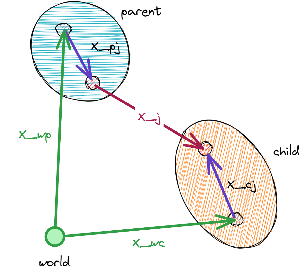
Symbol |
Description |
|---|---|
x_wp |
World transform of the parent body (stored at |
x_wc |
World transform of the child body (stored at |
x_pj |
Transform from the parent body to the joint parent anchor frame (defined by |
x_cj |
Transform from the child body to the joint child anchor frame (defined by |
x_j |
Joint transform from the joint parent anchor frame to the joint child anchor frame |
In the forward kinematics, the joint transform is determined by the joint coordinates (generalized joint positions State.joint_q and velocities State.joint_qd).
Given the parent body’s world transform \(x_{wp}\) and the joint transform \(x_{j}\), the child body’s world transform \(x_{wc}\) is computed as:
Newton’s public newton.eval_fk() writes State.body_qd using that
COM/world convention, and newton.eval_ik() expects the same convention
when recovering generalized state from maximal body state. For FREE,
DISTANCE, and ROD joints, the recovered generalized velocities are
rotated back into the joint parent frame.
- newton.eval_fk(model, joint_q, joint_qd, state, mask=None, indices=None, body_flag_filter=BodyFlags.ALL, *, joint_mask=None)[source]
Evaluates the model’s forward kinematics given the joint coordinates and updates the state’s body information (
State.body_qandState.body_qd).The written
State.body_qdvalues use Newton’s public body-twist convention(v_com_world, omega_world).To edit a branch while preserving the rest of a simulated articulation: refresh stale joint coordinates with
eval_ik()if needed, edit the desired joint coordinates, and pass ajoint_maskselecting the edited joint and all descendants that should follow it. UseModel.joint_ancestorto identify those descendants. Selecting only the edited joint leaves its descendants’ body poses and velocities unchanged.An
eval_ik()/ full FK round trip can change unrelated bodies when simulated poses or velocities do not exactly satisfy the joint constraints, as well as through numerical roundoff. The joint mask preserves unselected body state exactly instead of reconstructing it from joint coordinates.- Parameters:
model (Model) – The model to evaluate.
joint_q (wp.array[float]) – Generalized joint position coordinates, shape [joint_coord_count], float
joint_qd (wp.array[float]) – Generalized joint velocity coordinates, shape [joint_dof_count], float
state (State | Model | object) – The state-like target to update (e.g.,
StateorModel).mask (wp.array[bool] | None) – The mask to use to enable / disable FK for an articulation. If None then treat all as enabled, shape [articulation_count], bool
indices (wp.array[int] | None) – Integer indices of articulations to update. If None, updates all articulations. Cannot be used together with mask parameter.
body_flag_filter (int) – Body flag filter controlling which bodies are written to in
state.body_qandstate.body_qd. Default updates both dynamic and kinematic bodies. Bodies that do not match the filter retain their existing values; they are not zeroed or invalidated.joint_mask (wp.array[bool] | None) – Optional bool array on
model.device, shape [joint_count]. Only selected joints update their child bodies; unselected joints preserve the existing body pose and velocity. This only selects FK writes and is independent ofModel.joint_enabled. Selected joints use their parents’ current state, whether preserved or updated by this call. Descendants are not selected automatically: include them to propagate an edit through a branch. Intersects withmaskorindicesandbody_flag_filter. Supports autodiff and graph capture, including changes to mask values between graph replays.
- Raises:
ValueError – If both articulation filters are supplied, or
joint_maskhas the wrong dtype, shape, or device.
- newton.eval_ik(model, state, joint_q, joint_qd, mask=None, indices=None, body_flag_filter=BodyFlags.ALL)[source]
Evaluates the model’s inverse kinematics given the state’s body information (
State.body_qandState.body_qd) and updates the generalized joint coordinates joint_q and joint_qd.The input
State.body_qdis interpreted using Newton’s public body-twist convention(v_com_world, omega_world). For FREE, DISTANCE, and ROD joints, the recoveredjoint_qdlinear entries are referenced at the child COM and expressed in the joint parent frame.- Parameters:
model (Model) – The model to evaluate.
state (State | Model | object) – The state-like object with the body’s maximal coordinates (positions
State.body_qand velocitiesState.body_qd) to use.joint_q (wp.array[float]) – Generalized joint position coordinates, shape [joint_coord_count], float
joint_qd (wp.array[float]) – Generalized joint velocity coordinates, shape [joint_dof_count], float
mask (wp.array[bool] | None) – Boolean mask indicating which articulations to update. If None, updates all (or those specified by indices).
indices (wp.array[int] | None) – Integer indices of articulations to update. If None, updates all articulations.
body_flag_filter (int) – Body flag filter controlling which joints are written based on each joint’s child body flag. Default updates joints for both dynamic and kinematic child bodies. Entries that do not match the filter retain their existing values in
joint_qandjoint_qd.
Note
The mask and indices parameters are mutually exclusive. If both are provided, a ValueError is raised.
Inverse Dynamics#
Experimental
Experimental feature. API, behavior, defaults, and supported use cases may change without prior notice.
Newton can evaluate the manipulator equation for an articulated rigid-body system:
Symbol |
Description |
|---|---|
\(q\) |
Generalized joint coordinates ( |
\(\dot{q}\) |
Generalized joint velocities ( |
\(\ddot{q}\) |
Generalized joint accelerations (user-supplied |
\(\tau\) |
Generalized joint forces / torques, same layout as |
\(M(q)\) |
Joint-space mass matrix, shape |
\(g(q) = \partial U / \partial q\) |
Gravity force, where \(U(q) = \sum_i -m_i\, \mathbf{g} \cdot \mathbf{x}_{\text{com},i}\) is the system’s gravitational potential energy (sum over bodies of mass × gravity-vector · CoM position). Equivalently, the feed-forward joint-space force a controller must apply to hold the articulation static under gravity. |
\(C(q, \dot{q})\, \dot{q}\) |
Coriolis + centrifugal force. |
newton.eval_inverse_dynamics_passive() populates any requested
combination of \(M(q)\), \(g(q)\), and
\(C(q, \dot{q})\, \dot{q}\) into caller-allocated arrays. An output set to
None is not computed.
newton.eval_inverse_dynamics_force() then combines them with a
user-supplied \(\ddot{q}\) to produce \(\tau\).
Both functions require state.body_q to be consistent with
state.joint_q: callers must invoke newton.eval_fk() (or
otherwise update state.body_q) first.
# bring state.body_q in sync with state.joint_q (precondition of
# eval_inverse_dynamics_passive)
newton.eval_fk(model, state.joint_q, state.joint_qd, state)

# allocate the requested outputs
mass_matrix = wp.empty(
    (
        model.articulation_count,
        model.max_dofs_per_articulation,
        model.max_dofs_per_articulation,
    ),
    dtype=wp.float32,
    device=model.device,
)
gravity_force = wp.empty_like(state.joint_qd)
coriolis_force = wp.empty_like(state.joint_qd)
joint_f = wp.empty_like(state.joint_qd)

# populate M(q), g(q), and C(q, q_dot)*q_dot in one call
newton.eval_inverse_dynamics_passive(
    model,
    state,
    mass_matrix=mass_matrix,
    gravity_force=gravity_force,
    coriolis_force=coriolis_force,
)

# combine into the generalized joint force tau = M*joint_qdd + C*qdot + g
joint_qdd = wp.zeros_like(state.joint_qd)
newton.eval_inverse_dynamics_force(
    model,
    state,
    mass_matrix=mass_matrix,
    joint_qdd=joint_qdd,
    coriolis_force=coriolis_force,
    gravity_force=gravity_force,
    joint_f=joint_f,
)
Pass only the output arrays you need. For example, supplying
gravity_force= and coriolis_force= while leaving mass_matrix=None
skips the mass-matrix Jacobian pass.
Restricting evaluation with the selection API#
newton.selection.ArticulationView exposes
eval_inverse_dynamics_passive(), which
masks the computation to a label-matched (and optionally per-world)
subset of articulations. Output buffers stay sized for the whole model;
slots belonging to unselected articulations and DOFs come back as zero,
mirroring the convention newton.eval_mass_matrix() uses for its
own mask= argument.
# only compute M(q), g(q), and C*q_dot for selected articulations
view = newton.selection.ArticulationView(model, pattern="robot*")
view.eval_inverse_dynamics_passive(
    state,
    mass_matrix=mass_matrix,
    gravity_force=gravity_force,
    coriolis_force=coriolis_force,
)

# optionally narrow further with a per-world submask (shape [world_count])
per_world_mask = wp.array([True], dtype=bool, device=model.device)
view.eval_inverse_dynamics_passive(
    state,
    mass_matrix=mass_matrix,
    gravity_force=gravity_force,
    coriolis_force=coriolis_force,
    mask=per_world_mask,
)
The view also applies the same selection when combining the populated arrays with a desired acceleration:
view.eval_inverse_dynamics_force(
    state,
    mass_matrix=mass_matrix,
    joint_qdd=joint_qdd,
    coriolis_force=coriolis_force,
    gravity_force=gravity_force,
    joint_f=joint_f,
    mask=per_world_mask,
)
- newton.eval_inverse_dynamics_passive(model, state, *, mass_matrix=None, gravity_force=None, coriolis_force=None, mask=None)[source]
Compute passive inverse-dynamics quantities for articulated systems.
Only the non-
Noneoutputs are written; omitted outputs are not computed, although on CUDAgravity_forceandcoriolis_forceshare one pass. Callers allocate the requested output arrays:mass_matrix← the joint-space mass matrixM(q)[kg, kg·m, or kg·m^2, depending on the joint types of the row/column DOFs], withjoint_armatureadded to the diagonal;gravity_force← the gravity forceg(q) = ∂U/∂q[N or N·m, depending on joint type], whereU(q)is the system’s gravitational potential energysum_i -m_i * g . x_com_i. This is the joint-space force that holds the articulation static under gravity;coriolis_force← the Coriolis + centrifugal forceC(q, q_dot)*q_dot[N or N·m, depending on joint type].
All three quantities follow the standard manipulator-equation convention
tau = M(q)*joint_qdd + C(q,q_dot)*q_dot + g(q).Requires
state.body_qto be consistent withstate.joint_q; callers must invokeeval_fk()(or otherwise updatestate.body_q) before this function.Note
Inverse dynamics considers only the kinematic tree. As a consequence, loop-closure joints (
EqType.CONNECT,EqType.WELD,EqType.JOINT) play no role in the inverse dynamics evaluation.RODjoints are not supported by the inverse-dynamics pipeline.Experimental
Experimental feature. API, behavior, defaults, and supported use cases may change without prior notice.
- Parameters:
model (Model) – Model providing articulation topology and inertial parameters.
state (State) – State providing the current generalized coordinates and velocities.
state.body_qmust already reflectstate.joint_q.mass_matrix (wp.array3d[wp.float32] | None) – Optional output for the joint-space mass matrix, shape
(model.articulation_count, model.max_dofs_per_articulation,
model.max_dofs_per_articulation)
, dtype float. The padded rows and columns beyond each articulation’s DOF count are zero.gravity_force (wp.array[wp.float32] | None) – Optional output for
g(q) = ∂U/∂q[N or N·m, depending on joint type], shape(model.joint_dof_count,), dtype float.coriolis_force (wp.array[wp.float32] | None) – Optional output for
C(q, q_dot)*q_dot[N or N·m, depending on joint type], shape(model.joint_dof_count,), dtype float.mask (wp.array[bool] | None) – Optional
wp.array[bool]of shape(articulation_count,)selecting which articulations to compute. Entries belonging to unselected articulations are zero in the output buffers (mirroringeval_mass_matrix()’s mask convention). IfNone, all articulations are computed.
- Raises:
ValueError – If the model contains a
RODjoint, no outputs are requested, an output or mask has an unexpected shape, orgravity_forceandcoriolis_forceare the same array.
- newton.eval_inverse_dynamics_force(model, state, *, mass_matrix, joint_qdd, coriolis_force, gravity_force, joint_f, mask=None)[source]
Evaluate
tau = M(q)*joint_qdd + C(q,q_dot)*q_dot + g(q).Combines a per-articulation mass-matrix-times-acceleration product with the Coriolis and gravity forces to produce the full joint force required to realize
joint_qddat the current(q, q_dot)under gravity, writing the result tojoint_fin place. The two force inputs follow the standard manipulator-equation sign convention (+C(q,q_dot)*q_dotand+g(q) = +∂U/∂q, the buffers populated byeval_inverse_dynamics_passive()) and are added directly. Per-articulation DOF counts are recovered fromjoint_qd_start, so a mix of fixed-root and floating-root articulations across multiple worlds is handled uniformly.For any FREE/DISTANCE joint in the articulation tree, the mass matrix in
mass_matrixis expressed in the joint’s parent frame while the bias forces are in the world-frame CoM-wrench convention ofjoint_f. Each such joint’s mass-matrix-times-acceleration wrench is rotated to world (usingstate.body_qfor the parent-frame-in-world rotation) before the sum, sojoint_fis entirely in that world convention.RODjoints are not supported by the inverse-dynamics pipeline.Experimental
Experimental feature. API, behavior, defaults, and supported use cases may change without prior notice.
- Parameters:
model (Model) – The model containing articulation definitions.
state (newton.State) – State providing
body_q, used to rotate the FREE/DISTANCE root mass-matrix-times-acceleration wrench into the world frame. Must be consistent with the mass-matrix and bias-force buffers in this call (i.e. the state passed toeval_inverse_dynamics_passive()).mass_matrix (wp.array3d[wp.float32]) – Joint-space mass matrix, shape
(model.articulation_count, model.max_dofs_per_articulation,
model.max_dofs_per_articulation)
, dtype float. Entry units depend on the row and column DOF types: [kg] for two translational DOFs, [kg·m] for mixed translational/rotational DOFs, and [kg·m²] for two rotational DOFs.joint_qdd (wp.array[wp.float32]) – Generalized joint accelerations [m/s² or rad/s², depending on joint type], shape
(model.joint_dof_count,), dtype float.coriolis_force (wp.array[wp.float32]) – Coriolis + centrifugal force
C(q, q_dot)*q_dot[N or N·m, depending on joint type], shape(model.joint_dof_count,), dtype float.gravity_force (wp.array[wp.float32]) – Gravity force
g(q) = ∂U/∂q[N or N·m, depending on joint type], shape(model.joint_dof_count,), dtype float.joint_f (wp.array[wp.float32]) – Output generalized joint force :math:` au` [N or N·m, depending on joint type], shape
(model.joint_dof_count,), dtype float. Uses the same layout and convention asjoint_f.mask (wp.array[wp.bool] | None) – Optional
wp.array[bool]of shape(articulation_count,)selecting which articulations to compute. Unselected joint-force entries are zeroed without reading their mass-matrix, acceleration, or bias-force inputs.
- Raises:
ValueError – If the model contains a
RODjoint or an input, output, or mask has an unexpected shape.
Orphan joints#
A joint in one articulation cannot use a body from another articulation as its
parent. This cross-articulation topology is unsupported, and
finalize() rejects it. To compose imported assets with
add_urdf(), add_mjcf(), or
add_usd(), pass parent_body and base_joint so
the new joints are appended to the parent’s articulation.
An orphan joint is a joint that is not part of any articulation and whose child body is not reachable through any articulated joint (i.e. the child has no articulated path back to the rest of the model). This situation can arise when:
The USD asset does not define a
PhysicsArticulationRootAPIon any prim, so no articulations are discovered during parsing.A joint connects two bodies that are not under any
PhysicsArticulationRootAPIprim, even though other articulations exist in the scene.
A joint that is excluded from every add_articulation() call but whose two bodies are already reachable through the articulation tree is not an orphan joint; it is a loop-closing joint (see Loop closure) and is handled separately. A joint from world to a body is also allowed to remain outside articulation metadata as a standalone world-root joint.
USD import preserves joints outside authored articulations without emitting an articulation warning. The model’s validation and the selected solver determine whether the resulting topology is supported.
Validation and finalization
By default, finalize() raises a ValueError for joints that connect separate articulations and for non-root orphan joints. Loop-closing joints and standalone world-root joints pass this check. To proceed with either unsupported topology, set skip_validation_joints=True explicitly:
model = builder.finalize(skip_validation_joints=True)
Solver compatibility
Maximal-coordinate solvers (SolverXPBD, SolverSemiImplicit) consume joints independently of articulation membership. Semi-implicit joint constraints are penalty forces, so their accuracy and stability depend on the configured stiffness, damping, and time step.
SolverMuJoCo converts standalone world-root joints through a solver-specific fallback and emits a warning. It rejects general rootless mechanisms whose remaining bodies cannot be instantiated from articulations or standalone world roots. SolverFeatherstone requires reduced-coordinate articulation metadata.
Loop-closing joints are handled separately; see Loop closure.
Loop closure#
Newton’s add_joint_*() methods author kinematic
trees: each body has at most one parent joint, so the joints alone cannot
form a closed kinematic loop (for example a four-bar linkage or a parallel
mechanism). Closed loops must instead be expressed by declaring the topology
as a tree and adding a separate joint that re-couples the open end.
To close a loop, create the loop-closing joint with
add_joint_*() but omit it from the
``joint_list`` passed to add_articulation(),
so the articulation graph remains a tree. The omitted joint is a
loop-closing joint: its two bodies are both already reachable through
the tree, which distinguishes it from an
orphan joint (whose child has no articulated path
and which finalize() rejects unless
skip_validation_joints=True).
builder = newton.ModelBuilder()

# Fixed root attached to the world.
root = builder.add_link()
builder.add_shape_box(root, hx=0.1, hy=0.1, hz=0.1)
j_root = builder.add_joint_fixed(parent=-1, child=root)

# Child A: revolute about Z, hinged on the root at +X.
child_a = builder.add_link()
builder.add_shape_box(child_a, hx=0.5, hy=0.05, hz=0.05)
j_a = builder.add_joint_revolute(
    parent=root,
    child=child_a,
    axis=newton.Axis.Z,
    parent_xform=wp.transform(wp.vec3(1.0, 0.0, 0.0), wp.quat_identity()),
)

# Child B: revolute about Z, hinged on the root at -X.
child_b = builder.add_link()
builder.add_shape_box(child_b, hx=0.5, hy=0.05, hz=0.05)
j_b = builder.add_joint_revolute(
    parent=root,
    child=child_b,
    axis=newton.Axis.Z,
    parent_xform=wp.transform(wp.vec3(-1.0, 0.0, 0.0), wp.quat_identity()),
)

# Loop-closing joint: a fixed joint between the two children. Authored with
# add_joint_* exactly like a tree joint, but deliberately left out of the
# articulation below.
j_loop = builder.add_joint_fixed(parent=child_a, child=child_b)

# Only the tree joints (j_root, j_a, j_b) go into the articulation;
# j_loop is excluded so the articulation graph remains a tree.
builder.add_articulation([j_root, j_a, j_b])

model = builder.finalize()
Importing from USD. The same omit-from-articulation pattern is the
standard way UsdPhysics expresses loop closures, and Newton’s USD importer
honors it. Set the physics:excludeFromArticulation attribute to true
on a PhysicsJoint prim, and add_usd() will
register the joint with the builder via the normal add_joint_* path but
leave it out of the surrounding add_articulation()
call — producing exactly the topology shown above. This is how
a USD asset can author a four-bar linkage or other parallel mechanism.
Note
A loop-closing joint passes finalize()
validation by default — because its two bodies are already reachable
through the tree, the orphan-joint check does not fire and
skip_validation_joints=True is not required. Each solver then
handles the loop-closing joint differently:
Maximal-coordinate solvers track state as per-body transforms (
body_q/body_qd) and enforce joints as pairwise body constraints, so the loop-closure joint is solved alongside the tree joints with no special-casing. UnderSolverXPBDandSolverSemiImplicit,j_loopkeeps its full joint behavior — drive (joint_target_ke/joint_target_kd,control.joint_f) and joint limits are applied alongside the loop-closure constraint, subject to each solver’s general joint-feature support (see Joint Feature Support).SolverVBDandSolverKaminouse the same flat per-joint iteration but support a narrower set of joint types and features, so the same loop-closure pattern works only within their respective supported subsets.Generalized-coordinate solvers carry only tree-joint coordinates in their state vector and must handle the loop closure separately.
SolverMuJoCoenforces each loop-closure joint as a bilateral coupling at compile time, which restricts the supported joint types and drops joint-level features (see the note below).SolverSteelenforces loop-closing BALL, REVOLUTE, and FIXED joints as bilateral constraint rows (3, 5, and 6 rows) when the joint’s parent is in the same articulation, the world, or a kinematic body; other loop-closing joint types are rejected, and a loop-closing joint loses its drive and limits. Link-break loops keep every joint of the loop as a tree joint instead.SolverFeatherstonehas no such synthesis path: the loop-closure joint contributes no DOFs and the loop closure is silently not enforced.
In all cases the loop-closing joint is invisible to newton.eval_fk(),
newton.eval_ik(), and ArticulationView —
those walk the articulation tree only.
Note
SolverMuJoCo supports only a subset of joint
types as loop closures, and the loop-closing joint loses its joint-level
features (drive, limits, armature, friction). See
Loop closures for the supported types and MuJoCo-specific
behavior.
Link-break loops#
A loop-closing joint has no coordinate of its own, so generalized-coordinate
solvers cannot drive, limit, or mimic it. A link-break loop moves the cut
from a joint to a body instead (the approach of Drake’s SpanningForest):
one body of the loop is split into a primary and a shadow that share its
mass, the joint that would close the loop becomes a tree joint into the shadow,
and a FIXED loop-closing joint welds the shadow back to its primary. Every
joint of the loop, including the one that closes it, then keeps its
coordinate, drive, limits, and mimic relationships.
SolverSteel enforces the weld as six bilateral rows.
The four-bar below hinges a crank and a rocker on the world and splits the coupler that joins them:
builder = newton.ModelBuilder()
inertia = wp.mat33(0.02, 0.0, 0.0, 0.0, 0.02, 0.0, 0.0, 0.0, 0.02)
half_inertia = wp.mat33(0.01, 0.0, 0.0, 0.0, 0.01, 0.0, 0.0, 0.0, 0.01)

crank = builder.add_link(xform=wp.transform((0.0, 0.0, 0.5), wp.quat_identity()), mass=1.0, inertia=inertia)
rocker = builder.add_link(xform=wp.transform((1.0, 0.0, 0.5), wp.quat_identity()), mass=1.0, inertia=inertia)

# Split the coupler into a primary and a shadow at the same pose, each with
# half of its mass and inertia. Collision shapes go on the primary only.
coupler_pose = wp.transform((0.5, 0.0, 1.0), wp.quat_identity())
coupler = builder.add_link(xform=coupler_pose, mass=0.5, inertia=half_inertia)
coupler_shadow = builder.add_link(xform=coupler_pose, mass=0.5, inertia=half_inertia)


def hinge(parent, child, parent_pos, child_pos):
    return builder.add_joint_revolute(
        parent=parent,
        child=child,
        axis=newton.Axis.Y,
        parent_xform=wp.transform(parent_pos, wp.quat_identity()),
        child_xform=wp.transform(child_pos, wp.quat_identity()),
    )


j_a = hinge(-1, crank, (0.0, 0.0, 0.0), (0.0, 0.0, -0.5))
j_b = hinge(crank, coupler, (0.0, 0.0, 0.5), (-0.5, 0.0, 0.0))
j_d = hinge(-1, rocker, (1.0, 0.0, 0.0), (0.0, 0.0, -0.5))
# The hinge that closes the loop is a tree joint into the shadow, so it keeps its coordinate.
j_c = hinge(rocker, coupler_shadow, (0.0, 0.0, 0.5), (0.5, 0.0, 0.0))

# Both branches of the loop belong to one articulation.
builder.add_articulation([j_a, j_b, j_d, j_c])

# The weld is the loop-closing joint: it holds the shadow on its primary.
builder.add_joint_fixed(parent=coupler, child=coupler_shadow)

model = builder.finalize()
When building a link-break loop:
The primary and the shadow start at the same pose and keep the real body’s center of mass, and their masses and inertias add up to the real body’s (an even split is the usual choice). The weld’s two frames must coincide at the authored pose; identity frames do when the two bodies share a pose.
All tree joints of the loop, from both branches, go into one articulation, and the weld stays out of it. Steel rejects a weld between two dynamic articulations.
Cut on the far side of the loop from the articulation root so both branches stay short. Welding a long chain back onto its own root is valid but, in Steel, leaks more momentum.
With
SolverSteel, iterative weld rows converge slowly on spatial loops at low iteration counts.enable_bilateral_preeliminationsolves a weld directly when the articulation’s loop rows fit its capacity (8 rows, so one weld); larger models warn and fall back to iterative rows.Do not collapse fixed joints in a link-break model: build and import it with
collapse_fixed_joints=Falseand do not callcollapse_fixed_joints()afterwards. Collapsing merges the shadow into its primary or drops the weld, either of which opens the loop;collapse_fixed_joints()warns when it finds a weld closure.
The same structure can be authored in an asset:
MJCF: nest the shadow body (no geoms) inside the body that is the closing joint’s parent and give it the closing joint; give the primary and the shadow
<inertial>elements with the sameposand half of the mass and inertia each; and close the loop with<weld body1="coupler" body2="coupler_shadow"/>. Each top-level body of<worldbody>imports as its own articulation, so both branches must hang from one body there; for a loop on the ground, use a fixed base body without joints.USD: add the shadow as a rigid body with half of the mass properties, target the closing joint’s
physics:body1at it, and weld it to its primary with aPhysicsFixedJointwhosephysics:excludeFromArticulationistrue. Put both branches under one prim withPhysicsArticulationRootAPI.
Link-break welds and MuJoCo welds#
A link-break weld is a hard, topological loop closure. It plays the role of the
weld that Drake’s SpanningForest
adds between a split link’s primary and shadow, which Drake’s
MultibodyPlant enforces as a hard weld constraint. It is not a model of
MuJoCo’s soft <weld> equality, but the MJCF and USD importers convert MuJoCo
welds (<weld>, MjcEqualityWeldAPI) to the same loop joints:
torquescale0, which MuJoCo enforces as a point constraint with rotation free, becomes a BALL loop joint on the weld’s anchor, and the importer logs a warning.Any other
torquescalebecomes a FIXED loop joint. A value other than 1 logs a warning, because the weld is then enforced in full.SolverSteelsolves loop closures as hard constraints and does not supportsolreforsolimp(time constant, damping ratio, impedance) on them.SolverMuJoCoenforces the original equality row and keeps all of these parameters.
A link-break MJCF also runs in MuJoCo itself, where the weld is soft. To keep it close to a hard closure there:
Set the weld’s
solreftime constant to twicetimestepwith a damping ratio of 1, for examplesolref="0.002 1"withtimestep="0.001". MuJoCo raises smaller time constants to twice the timestep. With the defaultsolref(0.02 s), the weld of a four-bar’s coupler opens by about 1 mm and 0.6 degrees.Set
solimp="0.99 0.999 0.001"to raise the constraint impedance.Keep
torquescaleat its default of 1, and leaverelposeunset so the weld holds the authored pose.Leave the shadow without geoms, or exclude its contacts with the primary (
<contact><exclude body1="coupler" body2="coupler_shadow"/></contact>): MuJoCo skips collisions only between a parent and its child.For accuracy, use a smaller
timesteporintegrator="RK4".
Passive joint springs#
newton.Model.joint_stiffness and newton.Model.joint_rest_q
describe a passive joint spring. For each scalar coordinate, its generalized
force is stiffness * (rest_q - q). Passive damping adds
-joint_damping * qd. These forces act independently of the drive targets
and remain active when a joint limit is violated. The rest coordinate may
lie outside the limits to model preload.
Author scalar springs with newton.ModelBuilder.JointDofConfig or
the scalar joint helpers:
builder.add_joint_revolute(
    parent=-1, child=body, stiffness=2.0, rest_q=0.25,
    target_q=0.0, target_qd=0.0,
)
stiffness defaults to zero and has units N/m for linear axes and
N·m/rad for angular axes. The effective scalar rest coordinate defaults to zero
and is in meters or radians. JointDofConfig.rest_q=None leaves the coordinate
unspecified; finalization resolves it to zero unless a legacy spring input
supplies it. An explicitly configured zero takes precedence over a legacy
default and conflicts with an explicitly authored, different legacy rest.
target_q and target_qd configure drives;
target_pos and target_vel are deprecated aliases since Newton 1.8.
The stiffness array is DOF-sized. The rest array always has the same
coordinate layout as newton.Model.joint_q, including identity
quaternions (xyzw) for default rotational rest configurations. Index it
with newton.Model.joint_q_start. Scalar JointDofConfig.rest_q values cannot specify a
quaternion; edit the joint’s four entries in joint_rest_q instead.
Featherstone, Steel, and SemiImplicit apply springs only to REVOLUTE, PRISMATIC,
and D6 coordinates. MuJoCo
also supports isotropic BALL springs and quaternion rest orientations.
newton.solvers.SolverVBD uses joint_rest_q for ROD structural rest;
its material stiffness and damping remain in joint_target_ke / joint_target_kd.
Other solvers do not consume these properties yet. As with other model
features, unsupported springs do not produce automatic warnings; consult the
solver feature matrix when choosing a solver.
SemiImplicit derives angular coordinates from body orientations and does not
track multi-turn winding. Its scalar angular springs use a principal angle in
[-pi, pi), independent of quaternion sign. The displacement rest_q - q is
not wrapped, so rest coordinates outside that interval still produce preload.
However, crossing the -pi/pi boundary makes the coordinate jump by 2*pi and
the spring force jump by 2*pi*stiffness. This can destabilize motion even
near an equilibrium close to that boundary. Use Featherstone or MuJoCo, which
store unwrapped scalar joint coordinates, for boundary-crossing or multi-turn
motion. SemiImplicit winding support is tracked in
issue #4547.
MJCF stiffness and springref import into the core fields without explicit
solver custom-attribute registration.
For USD, reuse the existing MjcJointAPI mjc:stiffness,
mjc:springref, and mjc:ref properties with
newton.usd.SchemaResolverMjc enabled. This import path does not
require MuJoCo solver registration. NewtonJointAPI spring authoring
properties are tracked separately in issue #4516; no unregistered
Newton USD attributes are introduced here.
See Passive spring migration for reference-coordinate conversion, legacy attribute compatibility, and migration of runtime spring edits.
After runtime spring edits, call solver.notify_model_changed with
newton.ModelFlags.JOINT_DOF_PROPERTIES, or use
newton.ModelFlags.JOINT_DOF_FORCE_PROPERTIES for stiffness and
newton.ModelFlags.JOINT_REFERENCE_POSE_PROPERTIES for rest coordinates.
Modify existing arrays in place when reusing captured simulation graphs.