Download notebook View on GitHub Open in Colab

Newton Robotics 101: From Concepts to Manipulation

This notebook teaches Newton through a robotics workflow. First, you will create a small rigid-body scene, finalize it into a device-resident model, and step it with a solver. Then you will load a Franka robot, compare raw joint forces with joint position targets, and use inverse kinematics (IK) to produce arm targets from end-effector poses.

The examples stay small so each code cell has one main purpose. The final pick-and-place task reuses the same objects and loop structure introduced earlier: Model, State, Control, Contacts, solver substeps, IK objectives, and viewer logging.

🎬 See also the Newton hands-on lab from GTC 2026 that covered a similar version of this notebook.

Roadmap

1. Core concepts: ModelBuilder → Model → State / Control / Contacts → Solver

2. A tiny simulation: build a scene, allocate simulation buffers, and run a loop

3. Performance: use CUDA graph capture when running on GPU

4. Robot loading and raw actuation: load a Franka arm from URDF and write Control.joint_f

5. Joint targets: use Control.joint_target_q with PD gains for more predictable motion

6. IK path following: convert end-effector targets into joint targets

7. Manipulation: combine IK, contact, and gripper control in a Franka pick-and-place task

Setup and Imports

Newton uses Warp arrays and math types at the API boundary, so the notebook imports warp alongside newton. You will see Warp types such as wp.vec3, wp.transform, wp.quat, and wp.array when defining poses, targets, and simulation buffers.

numpy is used for host-side calculations, such as constructing target paths before copying them to Warp arrays. ViewerViser records the states logged by each simulation loop so the results can be replayed inside the notebook.

# Colab setup: install Newton before importing it.
import importlib.util
import subprocess
import sys

try:
    IN_COLAB = importlib.util.find_spec("google.colab") is not None
except ModuleNotFoundError:
    IN_COLAB = False

if IN_COLAB:
    subprocess.check_call([sys.executable, "-m", "pip", "install", "-q", "newton[notebook]"])

import numpy as np
import warp as wp

import newton
import newton.examples
import newton.ik as ik
import newton.utils

# Opt in to the coord-aligned target layout so joint_target_q matches joint_q.
newton.use_coord_layout_targets = True

wp.config.log_level = wp.LOG_WARNING

Utilities

The next cell contains notebook support code rather than Newton simulation logic. make_viewer() creates a Viser recorder for one output cell, render_mermaid() displays diagrams, and the progress-bar helpers avoid depending on notebook-specific tqdm behavior.

Set use_cpu = True only when you want to debug on CPU. The rest of the notebook assumes the default device, which is CUDA when a compatible GPU is available.

Core Concepts

Newton keeps simulation data split across explicit objects:

• ``ModelBuilder`` is the editable authoring object. It stores Python-side lists while you add bodies, shapes, joints, worlds, or imported assets.

• ``Model`` is the finalized description of the system. It owns device arrays for geometry, topology, joint parameters, material properties, and other data that normally stays fixed during a rollout.

• ``State`` stores values that change with time, including body transforms, velocities, forces, and generalized joint coordinates.

• ``Control`` stores inputs applied during stepping, such as generalized joint forces, position targets, velocity targets, and actuator inputs.

• ``Contacts`` stores the contact geometry generated for a particular state by the collision pipeline.

• ``Solver`` reads the model, input state, controls, contacts, and timestep, then writes the next state.

This layout makes ownership clear. The model can be shared by many states, controls can be changed without rebuilding the model, and contact generation can be swapped or configured separately from the solver that consumes the contacts.

Newton is based on NVIDIA Warp

Newton solvers and collision routines launch Warp kernels internally. This tutorial does not require you to write custom kernels, but the public API still uses Warp data structures for device arrays, vectors, transforms, quaternions, and CUDA graph capture.

The first launch of a new Warp kernel specializes and compiles code for the argument types and target device. That compilation cost explains much of the delay the first time a simulation cell runs. After compilation, Warp reuses cached kernels for later calls with the same signature.

warp_workflow_diagram = r"""
flowchart TD
    K["Write @wp.kernel in Python"]
    L["First wp.launch(..., device='cuda')"]

    subgraph JIT["Warp JIT"]
        AST["Parse kernel + types"]
        CU["Generate CUDA C++"]
        NV["Compile with NVRTC/NVCC"]
    end

    RUN["Run kernel on GPU"]

    K --> L --> AST --> CU --> NV --> RUN
"""

render_mermaid(warp_workflow_diagram, theme="forest", line_color="#76b900", width="50%")

flowchart TD
    K["Write @wp.kernel in Python"]
    L["First wp.launch(..., device='cuda')"]

    subgraph JIT["Warp JIT"]
        AST["Parse kernel + types"]
        CU["Generate CUDA C++"]
        NV["Compile with NVRTC/NVCC"]
    end

    RUN["Run kernel on GPU"]

    K --> L --> AST --> CU --> NV --> RUN

1) From ModelBuilder to Model

We start with a scene that has one static shape and two dynamic rigid bodies. add_ground_plane() creates a world-attached plane. add_body() creates a rigid body that can move under forces, contacts, and gravity, and returns the body index. The add_shape_*() calls attach collision geometry to a body.

The xform argument is a Warp transform: translation plus quaternion rotation. For boxes, hx, hy, and hz are half-extents in meters, so hx=0.15 produces a box that is 0.30 m wide along that local axis.

core_concepts_diagram = r"""
flowchart LR
    subgraph Input["Input Data"]
        M[newton.Model]
        S[newton.State]
        C[newton.Control]
        K[newton.Contacts]
        DT[Time step dt]
    end

    STEP["solver.step()"]

    subgraph Output["Output Data"]
        SO["newton.State (updated)"]
    end

    %% Connections
    M --> STEP
    S --> STEP
    C --> STEP
    K --> STEP
    DT --> STEP
    STEP --> SO
"""

render_mermaid(core_concepts_diagram, theme="forest", line_color="#76b900")

flowchart LR
    subgraph Input["Input Data"]
        M[newton.Model]
        S[newton.State]
        C[newton.Control]
        K[newton.Contacts]
        DT[Time step dt]
    end

    STEP["solver.step()"]

    subgraph Output["Output Data"]
        SO["newton.State (updated)"]
    end

    %% Connections
    M --> STEP
    S --> STEP
    C --> STEP
    K --> STEP
    DT --> STEP
    STEP --> SO

builder = newton.ModelBuilder()

# Static ground (body=-1 means it's attached to the world, i.e. static)
builder.add_ground_plane()

# Dynamic box - add_body() returns the body index, which we pass to add_shape_*()
box_body = builder.add_body(xform=wp.transform(wp.vec3(0.0, -1.0, 1.0), wp.quat_identity()))
builder.add_shape_box(box_body, hx=0.15, hy=0.15, hz=0.15)

# Dynamic sphere
sphere_body = builder.add_body(xform=wp.transform(wp.vec3(0.0, 1.0, 1.2), wp.quat_identity()))
builder.add_shape_sphere(sphere_body, radius=0.18)

print(f"Bodies: {builder.body_count}, Shapes: {builder.shape_count}")

Bodies: 2, Shapes: 3

The count should show two dynamic bodies and three shapes. The ground plane contributes a shape attached to the world, while the box and sphere each contribute one body and one attached shape.

Finalize into Model, State, Control, Contacts

finalize() converts the builder’s Python lists into a Model with Warp arrays on the selected device. After finalization, allocate runtime objects from the model:

• model.state() clones the model’s initial positions and velocities into a new State.

• Two states are used because the solver reads from one state and writes into another.

• model.control() creates control arrays initialized from the model’s default control values.

• model.contacts() allocates a reusable contact buffer for the model’s collision pipeline.

Construct these objects through the model rather than by calling their classes directly. The model knows which arrays are needed for the scene that was built.

# finalize() compiles the builder into a device-ready Model
model = builder.finalize()

# Allocate two State buffers (we ping-pong between them during simulation)
state_0 = model.state()
state_1 = model.state()
control = model.control()
contacts = model.contacts()

print(f"Model device: {model.device}")
print(f"Body count: {model.body_count}")

viewer = make_viewer("tiny_model")
viewer.set_model(model)
viewer.log_state(state_0)
viewer

Model device: cpu
Body count: 2

╭────── viser (listening *:8080) ───────╮
│             ╷                         │
│   HTTP      │ http://localhost:8080   │
│   Websocket │ ws://localhost:8080     │
│             ╵                         │
╰───────────────────────────────────────╯

Note: orbit the camera by dragging with the left mouse button. Drag with the right mouse button to pan, and use the mouse wheel to zoom.

2) Solver and Simulation Loop

This first scene uses SolverXPBD, an implicit XPBD solver that supports rigid bodies, contacts, and several soft-body features. The later Franka examples use SolverMuJoCo because that solver operates on articulated robots in generalized coordinates and supports the joint target settings used below.

Each substep follows the same data flow:

1. state_0.clear_forces() resets external force accumulators on the input state.

2. model.collide(state_0, contacts) computes contacts from the current body poses and writes them into contacts.

3. solver.step(...) integrates one timestep from state_0 to state_1 using the current controls and contacts.

4. The two state references are swapped so the next substep starts from the newest state.

A rendered frame is split into several smaller solver timesteps. Smaller sim_dt values usually improve contact and controller stability, at the cost of more solver work per frame.

solver = newton.solvers.SolverXPBD(model, iterations=10)

fps = 60
frame_dt = 1.0 / fps
sim_substeps = 8
sim_dt = frame_dt / sim_substeps


def simulate():
    """Run one frame of simulation (multiple substeps)."""
    global state_0, state_1

    for _ in range(sim_substeps):
        state_0.clear_forces()
        model.collide(state_0, contacts)
        solver.step(state_in=state_0, state_out=state_1, control=control, contacts=contacts, dt=sim_dt)
        # Swap buffers so state_0 always holds the latest state
        state_0, state_1 = state_1, state_0

Visualize the First Simulation

The viewer records the state after each rendered frame. begin_frame(sim_time) and end_frame() define the timestamped frame in the recording; log_state(state_0) stores body and shape transforms for that frame.

The first run may spend most of its time compiling Warp kernels. The progress bar advances after compilation reaches the repeated simulation loop.

viewer = make_viewer("01_simple_scene")
viewer.set_model(model)

print("Starting simulation, this may take a minute or longer to compile the CUDA kernels...")

sim_time = 0.0
num_frames = 180
for _ in trange(num_frames):
    simulate()
    viewer.begin_frame(sim_time)
    viewer.log_state(state_0)
    viewer.end_frame()
    sim_time += frame_dt

viewer

╭────── viser (listening *:8081) ───────╮
│             ╷                         │
│   HTTP      │ http://localhost:8081   │
│   Websocket │ ws://localhost:8081     │
│             ╵                         │
╰───────────────────────────────────────╯

Starting simulation, this may take a minute or longer to compile the CUDA kernels...

3) Performance: CUDA Graph Capture

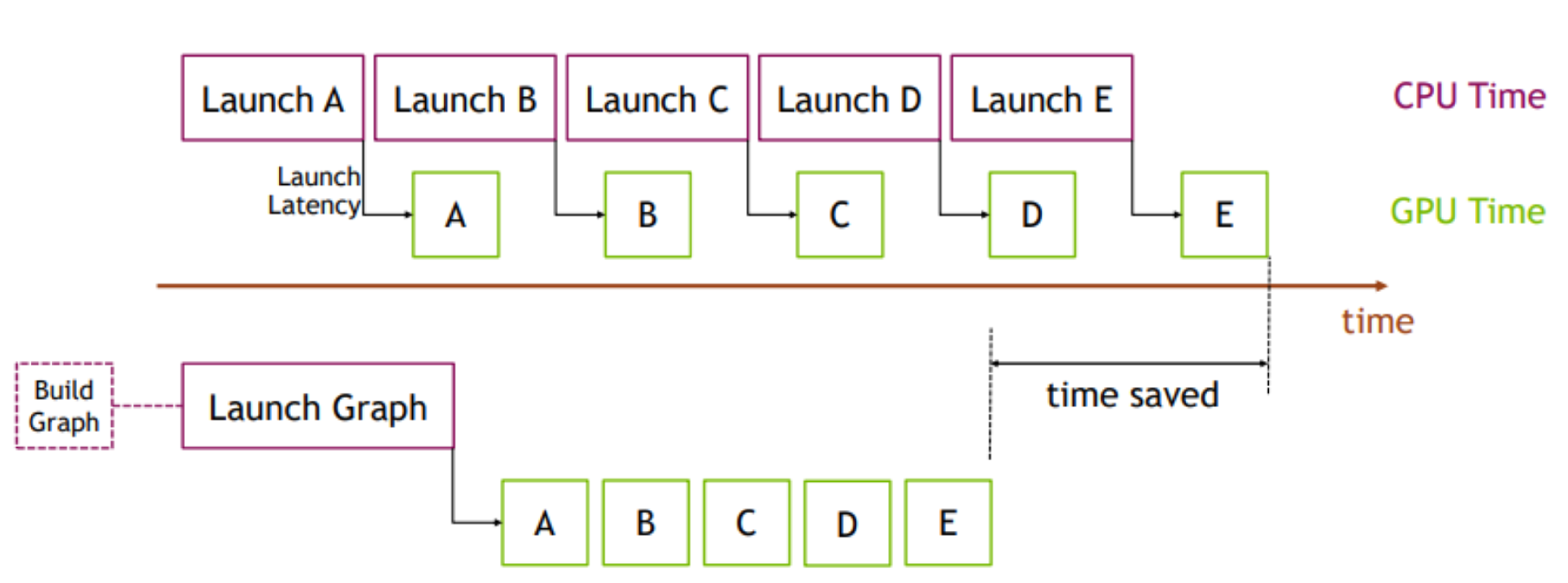
A frame with eight substeps launches many kernels: force clearing, collision detection, constraint solving, integration, and buffer updates. On CUDA, Python launch overhead can become visible when those kernels are short.

CUDA graph capture records the sequence of GPU operations and the device buffers they use. Replaying the graph submits that recorded sequence with less launch overhead. The contents of state_0, state_1, control, and contacts may change between replays, but the captured graph still refers to the same allocated buffers. Rebuild the graph if you reallocate those buffers or change the model structure.

# NOTE: CUDA graphs capture the exact GPU operations in simulate() as a replayable graph.
# Do not reallocate state_0/state_1 after capture - the graph references those specific buffers.
graph = None
if wp.get_device().is_cuda:
    with wp.ScopedCapture() as capture:
        simulate()
    graph = capture.graph
    print("CUDA graph captured - kernel launches are now batched into a single replay")
else:
    print("Running on CPU; graph capture skipped")

Running on CPU; graph capture skipped

The next two cells run the same number of frames with and without graph replay. Treat the numbers as a local timing check rather than a benchmark: they depend on the GPU, driver, and whether kernels were already compiled.

if wp.get_device().is_cuda:
    with wp.ScopedTimer("without_graph_capture"):
        for _ in range(120):
            simulate()

if graph is not None:
    with wp.ScopedTimer("with_graph_capture"):
        for _ in range(120):
            wp.capture_launch(graph)

4) Load a Robot and Apply Joint Forces

The Franka examples use ModelBuilder.add_urdf() instead of manually adding every link and joint. We will keep the setup in small pieces so the control choices stay visible: first define the robot constants, then build the physical scene, then choose how the joints are driven.

Important setup choices:

• floating=False fixes the robot base to the world instead of adding a free base joint.

• enable_self_collisions=False disables collisions between robot links for this tutorial scene.

• parse_visuals_as_colliders=False uses collision geometry from the URDF rather than treating visual meshes as colliders.

• FRANKA_HOME_Q contains 7 arm joint positions in radians and 2 finger positions in meters. The finger limits in this URDF are [0.0, 0.04] m, so the notebook uses 0.04 for open and 0.0 for closed.

• newton.eval_fk(...) updates body transforms from the initialized generalized coordinates before visualization or contact generation.

The URDF supplies joint limits, masses, inertias, and effort limits. The small armature values below are a simulation choice for SolverMuJoCo: they add diagonal inertia to the controlled DOFs, which helps regularize the articulated solve.

FRANKA_FINGER_CLOSED = 0.0
FRANKA_FINGER_OPEN = 0.04

# Franka initial joint positions (7 arm joints [rad] + 2 gripper fingers [m])
FRANKA_HOME_Q = [
    0.0,
    0.02,
    0.0,
    -2.37,
    0.0,
    2.39,
    np.pi / 4,
    FRANKA_FINGER_OPEN,
    FRANKA_FINGER_OPEN,
]

FRANKA_DOF_COUNT = 9
FRANKA_ARM_DOF_COUNT = 7

# These values set controller limits and solver regularization for the first 9 Franka DOFs.
FRANKA_EFFORT_LIMITS = [87, 87, 87, 87, 12, 12, 12, 100, 100]
FRANKA_MUJOCO_ARMATURE = [0.195] * 4 + [0.074] * 3 + [0.1] * 2

Build the Franka Scene

build_franka_scene() only creates the physical model: optional table, Franka URDF, initial joint coordinates, effort limits, armature, and optional cube. It does not enable the PD target controller. That separation lets each later section show the exact controller setup it needs.

SolverMuJoCo.register_custom_attributes(builder) declares MuJoCo-specific arrays before assets are loaded. Some examples below author values into those arrays before builder.finalize() creates the device-side Model.

def build_franka_scene(include_table=True, include_cube=True):
    """Build a Franka + table scene and optionally add a cube.

    Args:
        include_table: Whether to add a table.
        include_cube: Whether to add a cube on the table.

    Returns:
        Tuple of (builder, cube_size, table_pos, cube_body).
    """
    builder = newton.ModelBuilder()
    builder.default_shape_cfg.gap = 0.0
    newton.solvers.SolverMuJoCo.register_custom_attributes(builder)

    table_height = 0.1
    table_pos = wp.vec3(0.0, -0.5, 0.5 * table_height)
    table_top_center = table_pos + wp.vec3(0.0, 0.0, 0.5 * table_height)
    if include_table:
        builder.add_shape_box(
            body=-1,
            hx=0.4,
            hy=0.4,
            hz=0.5 * table_height,
            xform=wp.transform(table_pos),
        )

    robot_base_pos = table_top_center + wp.vec3(-0.5, 0.0, 0.0)
    builder.add_urdf(
        str(newton.utils.download_asset("franka_emika_panda") / "urdf/fr3_franka_hand.urdf"),
        xform=wp.transform(robot_base_pos, wp.quat_identity()),
        floating=False,
        enable_self_collisions=False,
        parse_visuals_as_colliders=False,
    )

    builder.joint_q[:FRANKA_DOF_COUNT] = FRANKA_HOME_Q
    builder.joint_effort_limit[:FRANKA_DOF_COUNT] = FRANKA_EFFORT_LIMITS
    builder.joint_armature[:FRANKA_DOF_COUNT] = FRANKA_MUJOCO_ARMATURE

    cube_size = 0.05
    cube_body = None
    if include_cube:
        cube_pos = table_top_center + wp.vec3(0.0, 0.15, 0.5 * cube_size)
        cube_body = builder.add_body(xform=wp.transform(cube_pos, wp.quat_identity()))
        shape_cfg = newton.ModelBuilder.ShapeConfig(margin=1e-3, density=400.0)
        builder.add_shape_box(
            body=cube_body,
            hx=0.5 * cube_size,
            hy=0.5 * cube_size,
            hz=0.5 * cube_size,
            cfg=shape_cfg,
        )

    return builder, cube_size, table_pos, cube_body

Raw Force Scene

For the first robot example we do not author any target positions or target gains. Position target control is opt-in in this course: the notebook adds joint_target_q, joint_target_ke, and joint_target_kd later, when it switches to target control. The next simulation loop writes directly to Control.joint_f.

# Build a scene without a cube; this section drives one joint with raw force.
builder, _, _, _ = build_franka_scene(include_cube=False)

model = builder.finalize()

state_0 = model.state()
state_1 = model.state()
control = model.control()
contacts = model.contacts()

# Forward kinematics: compute body transforms from the initial joint_q.
newton.eval_fk(model, model.joint_q, model.joint_qd, state_0)

viewer = make_viewer("02_franka_scene")
viewer.set_model(model)
viewer.set_camera(wp.vec3(0.5, 0.0, 0.5), -15, -140)
viewer.begin_frame(0)
viewer.log_state(state_0)
viewer.end_frame()
viewer

Cloning https://github.com/newton-physics/newton-assets.git (ref: 8e8df07d2e4829442d3d3d3aeecee1857f9951d7)...
Successfully downloaded folder to: /home/runner/.cache/newton/newton-assets_franka_emika_panda_d2ca1ca1_8e8df07d/franka_emika_panda

╭────── viser (listening *:8082) ───────╮
│             ╷                         │
│   HTTP      │ http://localhost:8082   │
│   Websocket │ ws://localhost:8082     │
│             ╵                         │
╰───────────────────────────────────────╯

After this cell, the viewer should show the imported Franka at its initial joint configuration. Later sections call build_franka_scene() again so each example starts from a clean builder, then applies the controller setup directly before finalize().

Now apply a sinusoidal generalized force to one arm degree of freedom.

Control.joint_f has one value per generalized velocity coordinate, in the same order as State.joint_qd. For a revolute joint, the value is a torque. In this section the joint target gains are zero, so only the commanded torque and passive dynamics affect the arm. The resulting motion is not meant to be a good controller; it shows the low-level force interface.

SolverMuJoCo is configured with use_mujoco_contacts=False, so contacts come from Newton’s collision pipeline. Each substep calls model.collide(state_0, contacts), and the populated Contacts object is passed to solver.step(...).

solver = newton.solvers.SolverMuJoCo(
    model,
    solver="newton",  # Constraint solver ("cg" or "newton")
    integrator="implicitfast",  # Integration method ("euler", "rk4", "implicit", "implicitfast")
    iterations=20,  # Number of solver iterations
    ls_iterations=100,  # Number of line-search iterations
    nconmax=1000,  # Maximum number of contact points per world
    njmax=2000,  # Maximum number of constraints per world
    cone="elliptic",  # Contact friction cone ("pyramidal" or "elliptic")
    impratio=1000.0,  # Frictional-to-normal constraint impedance ratio
    use_mujoco_contacts=False,  # Use Newton contacts instead of MuJoCo contacts
)

fps = 60
frame_dt = 1.0 / fps
sim_substeps = 8
sim_dt = frame_dt / sim_substeps

viewer = make_viewer("03_franka_joint_forces")
viewer.set_model(model)
viewer.set_camera(wp.vec3(0.5, 0.0, 0.5), -15, -140)

num_frames = 180
sim_time = 0.0
graph = None

print("Beginning simulation - it may take a minute or longer to compile the MuJoCo-Warp kernels...")


def run_sim_substeps():
    global state_0, state_1
    for _ in range(sim_substeps):
        state_0.clear_forces()
        model.collide(state_0, contacts)
        solver.step(state_in=state_0, state_out=state_1, control=control, contacts=contacts, dt=sim_dt)
        state_0, state_1 = state_1, state_0


for frame in trange(num_frames):
    # Apply a sinusoidal torque to the elbow joint (index 2)
    joint_forces = np.zeros(model.joint_dof_count, dtype=np.float32)
    joint_forces[2] = 35.0 * np.sin(2.0 * np.pi * frame / num_frames)
    control.joint_f.assign(joint_forces)

    # Capture CUDA graph on first frame, then replay
    if graph is not None:
        wp.capture_launch(graph)
    elif wp.get_device().is_cuda:
        with wp.ScopedCapture() as capture:
            run_sim_substeps()
        graph = capture.graph
    else:
        run_sim_substeps()

    viewer.begin_frame(sim_time)
    viewer.log_state(state_0)
    viewer.end_frame()
    sim_time += frame_dt

viewer

╭────── viser (listening *:8083) ───────╮
│             ╷                         │
│   HTTP      │ http://localhost:8083   │
│   Websocket │ ws://localhost:8083     │
│             ╵                         │
╰───────────────────────────────────────╯

Beginning simulation - it may take a minute or longer to compile the MuJoCo-Warp kernels...

5) Joint Targets with Control.joint_target_q

Joint position targets are the next control level up from raw forces. The model stores the per-DOF gains (joint_target_ke and joint_target_kd), while the control object stores target values that can change every frame.

The setup is easiest to follow when the target-controller code is next to the explanation:

• builder.joint_target_q[:9] = FRANKA_HOME_Q assigns the initial joint coordinate targets (matching Control.joint_target_q’s coord layout).

• builder.joint_target_ke and builder.joint_target_kd set the PD gains that will be stored on the finalized Model.

• mujoco:gravcomp is a per-body MuJoCo attribute. Setting it to 1.0 on the imported Franka links cancels their weight in MuJoCo’s gravity compensation path.

• mujoco:jnt_actgravcomp is a per-DOF MuJoCo attribute that maps to MuJoCo’s actuatorgravcomp joint flag. Setting it on the controlled DOFs makes the generated MuJoCo model include gravity compensation on those actuated joint coordinates.

With the static gravitational load handled separately, the PD gains can be lower: they mainly correct tracking error instead of also holding the arm up. Effort limits still cap the torque or force at each DOF.

FRANKA_TARGET_KE = [900, 900, 700, 700, 400, 400, 400, 100, 100]
FRANKA_TARGET_KD = [90, 90, 70, 70, 40, 40, 40, 10, 10]
FRANKA_BODY_GRAVCOMP = 1.0


def enable_franka_target_control(builder):
    """Enable position targets and MuJoCo gravity compensation for Franka."""
    builder.joint_target_q[:FRANKA_DOF_COUNT] = FRANKA_HOME_Q
    builder.joint_target_ke[:FRANKA_DOF_COUNT] = FRANKA_TARGET_KE
    builder.joint_target_kd[:FRANKA_DOF_COUNT] = FRANKA_TARGET_KD

    joint_actgravcomp = builder.custom_attributes["mujoco:jnt_actgravcomp"].values
    for dof_index in range(FRANKA_DOF_COUNT):
        joint_actgravcomp[dof_index] = True

    body_gravcomp = builder.custom_attributes["mujoco:gravcomp"].values
    for body_index, label in enumerate(builder.body_label):
        # Skip the world-fixed base bodies; compensate the moving arm, hand, and fingers.
        if label.startswith("fr3/") and label not in {"fr3/base", "fr3/fr3_link0"}:
            body_gravcomp[body_index] = FRANKA_BODY_GRAVCOMP

The next cell uses that helper immediately: build the scene, enable target control, then finalize. After model.control() is created, the loop only changes control.joint_target_q; the gains and MuJoCo attributes remain fixed on the Model.

builder, _, _, _ = build_franka_scene(include_cube=False)
enable_franka_target_control(builder)
model = builder.finalize()

state_0 = model.state()
state_1 = model.state()
control = model.control()
contacts = model.contacts()

# Same solver setup as before - see section 4 for parameter descriptions
solver = newton.solvers.SolverMuJoCo(
    model,
    solver="newton",
    integrator="implicitfast",
    iterations=20,
    ls_iterations=100,
    nconmax=1000,
    njmax=2000,
    cone="elliptic",
    impratio=1000.0,
    use_mujoco_contacts=False,
)

newton.eval_fk(model, model.joint_q, model.joint_qd, state_0)

fps = 60
frame_dt = 1.0 / fps
sim_substeps = 8
sim_dt = frame_dt / sim_substeps

viewer = make_viewer("04_franka_joint_targets")
viewer.set_model(model)
viewer.set_camera(wp.vec3(0.5, 0.0, 0.5), -15, -140)

base_target = model.joint_q.numpy().astype(np.float32)
base_target[FRANKA_ARM_DOF_COUNT:FRANKA_DOF_COUNT] = (
    FRANKA_FINGER_OPEN  # gripper finger targets stay within [0.0, 0.04] m
)

num_frames = 180
sim_time = 0.0
graph = None


def run_sim_substeps():
    global state_0, state_1
    for _ in range(sim_substeps):
        state_0.clear_forces()
        model.collide(state_0, contacts)
        solver.step(state_in=state_0, state_out=state_1, control=control, contacts=contacts, dt=sim_dt)
        state_0, state_1 = state_1, state_0


for frame in trange(num_frames):
    # Oscillate joint 3 (shoulder/elbow) around its home position.
    target = base_target.copy()
    target[3] = base_target[3] + 0.4 * np.sin(2.0 * np.pi * frame / num_frames)
    control.joint_target_q.assign(target)

    if graph is not None:
        wp.capture_launch(graph)
    elif wp.get_device().is_cuda:
        with wp.ScopedCapture() as capture:
            run_sim_substeps()
        graph = capture.graph
    else:
        run_sim_substeps()

    viewer.begin_frame(sim_time)
    viewer.log_state(state_0)
    viewer.end_frame()
    sim_time += frame_dt

viewer

╭────── viser (listening *:8084) ───────╮
│             ╷                         │
│   HTTP      │ http://localhost:8084   │
│   Websocket │ ws://localhost:8084     │
│             ╵                         │
╰───────────────────────────────────────╯

Inverse Kinematics (IK) in Newton

Joint targets require joint coordinates. Manipulation tasks are often easier to specify in task space: a point on the gripper should be at a world-space position, and the gripper frame should have a chosen orientation. Inverse kinematics converts those task-space targets into joint coordinates.

Newton’s IK module newton.ik is a GPU-first, batched IK system built on Warp. “Batched” means one IKSolver can solve many independent IK problems at once, for example many robots or many candidate targets. Each problem is defined by a set of objectives. An objective contributes residuals, which are error terms the optimizer tries to reduce:

• IKObjectivePosition measures the error between a point on a link and a target position [m].

• IKObjectiveRotation measures orientation error for a link frame.

• IKObjectiveJointLimit adds residuals only when joint coordinates move outside configured limits.

IKSolver also lets you choose how the solve is carried out:

• Optimizer: LM (Levenberg-Marquardt) or LBFGS. LM is the default used below and is a common choice for least-squares IK problems.

• Jacobian backend: ANALYTIC, AUTODIFF, or MIXED. A Jacobian tells the optimizer how each joint affects each residual. Analytic Jacobians are hand-derived and fast for built-in objectives; autodiff is more general; mixed mode uses analytic rows where available and autodiff elsewhere.

• Sampling: NONE, GAUSS, UNIFORM, or ROBERTS. IK can converge to different local solutions depending on the starting joint configuration. With multiple seeds, Newton optimizes several starting guesses in parallel and keeps the lowest-cost result.

The examples below use one IK problem, one seed, LM, and analytic Jacobians so the data flow is easy to see. For large batches, the same API can solve many IK targets in parallel, and repeated solves can be captured in CUDA graphs. The PR that introduced the IK module includes benchmark tables over 2M samples comparing Newton against PyRoki and cuRobo on Franka and H1 tasks: newton-physics/newton#394. In that setup, Newton reports 99.994% success on Franka and 99.996% on H1, with lower batch solve times than the listed baselines. Treat those numbers as benchmark context, not a guarantee for every robot or objective set.

ik_module_diagram = r"""
flowchart TD

    IKS[IKSolver]

    IKS --> OBJ[Objectives]
    OBJ --> O1[Position]
    OBJ --> O2[Rotation]
    OBJ --> O3[JointLimit]

    IKS --> OPT[Optimizer]
    OPT --> OPT1[Levenberg-Marquardt]
    OPT --> OPT2[LBFGS]

    IKS --> JAC[Jacobian mode]
    JAC --> J1[ANALYTIC]
    JAC --> J2[AUTODIFF]
    JAC --> J3[MIXED]

    IKS --> SMP[Sampling]
    SMP --> S1[NONE]
    SMP --> S2[GAUSS]
    SMP --> S3[UNIFORM]
    SMP --> S4[ROBERTS]
"""

render_mermaid(ik_module_diagram, theme="forest", line_color="#76b900")

flowchart TD

    IKS[IKSolver]

    IKS --> OBJ[Objectives]
    OBJ --> O1[Position]
    OBJ --> O2[Rotation]
    OBJ --> O3[JointLimit]

    IKS --> OPT[Optimizer]
    OPT --> OPT1[Levenberg-Marquardt]
    OPT --> OPT2[LBFGS]

    IKS --> JAC[Jacobian mode]
    JAC --> J1[ANALYTIC]
    JAC --> J2[AUTODIFF]
    JAC --> J3[MIXED]

    IKS --> SMP[Sampling]
    SMP --> S1[NONE]
    SMP --> S2[GAUSS]
    SMP --> S3[UNIFORM]
    SMP --> S4[ROBERTS]

6) IK Path Following

This section introduces IK objectives one at a time. Every solve includes the joint-limit objective so the returned joint coordinates stay inside the Franka limits stored on the model.

Target arrays are batched. This notebook uses n_problems=1, so each target array contains one entry, but the same API can solve many IK problems in parallel.

The code is intentionally repeated for the first few cells. Repetition keeps the objective construction, target updates, IK solve, and control copy visible before the final section wraps them in helpers.

1. Solve a single position target using position plus joint limits.

2. Add a rotation target to the same single-point task.

3. Preview a rectangle target path without IK.

4. Track the full rectangle with IK.

Step 1: Position-Only IK on One Target

The first IK task controls one point on the end-effector link. link_index=11 is the end-effector body index for this imported Franka asset. link_offset=wp.vec3(0.0, 0.0, 0.0) means the controlled point is the link frame origin.

Because this solve has no orientation objective, the end-effector may rotate while reaching the target point. The starting configuration and joint-limit objective still influence which joint configuration the optimizer finds.

builder, _, _, _ = build_franka_scene(include_table=False, include_cube=False)
enable_franka_target_control(builder)
model = builder.finalize()

state_0 = model.state()
state_1 = model.state()
control = model.control()
contacts = model.contacts()

solver = newton.solvers.SolverMuJoCo(
    model,
    solver="newton",
    integrator="implicitfast",
    iterations=20,
    ls_iterations=100,
    nconmax=500,
    njmax=1000,
    cone="elliptic",
    impratio=1000.0,
)

newton.eval_fk(model, model.joint_q, model.joint_qd, state_0)

fps = 60
frame_dt = 1.0 / fps
sim_substeps = 8
sim_dt = frame_dt / sim_substeps

ee_index = 11  # end-effector body index in the Franka model
home_pos_np = state_0.body_q.numpy()[ee_index][:3].astype(np.float32)
single_target_np = home_pos_np + np.array([0.0, 0.52, 0.04], dtype=np.float32)

The position objective below says which point should move where. The joint-limit objective does not pull the robot toward a preferred pose; it only adds residuals when a candidate solution moves outside the configured limits.

pos_obj = ik.IKObjectivePosition(
    link_index=ee_index,
    link_offset=wp.vec3(0.0, 0.0, 0.0),
    target_positions=wp.array([single_target_np], dtype=wp.vec3),
)

joint_limit_obj = ik.IKObjectiveJointLimit(
    joint_limit_lower=model.joint_limit_lower,
    joint_limit_upper=model.joint_limit_upper,
)

joint_q_ik = wp.clone(model.joint_q.reshape((1, -1)))
ik_solver = ik.IKSolver(
    model=model,
    n_problems=1,
    objectives=[pos_obj, joint_limit_obj],
    lambda_initial=0.1,
    jacobian_mode=ik.IKJacobianType.ANALYTIC,
)

Each frame solves IK from the previous IK solution, copies the first seven coordinates into the arm targets, keeps the fingers closed, and advances the physics state. The trace is logged from the simulated end-effector position, not from the requested target.

viewer = make_viewer("05_franka_ik_single_position")
viewer.set_model(model)
viewer.set_camera(wp.vec3(0.5, 0.0, 0.5), -15, -140)

sim_time = 0.0
ee_trace = []
graph = None


def run_sim_substeps():
    global state_0, state_1
    for _ in range(sim_substeps):
        state_0.clear_forces()
        solver.step(state_in=state_0, state_out=state_1, control=control, contacts=contacts, dt=sim_dt)
        state_0, state_1 = state_1, state_0


for _ in trange(120):
    pos_obj.set_target_positions(wp.array([single_target_np], dtype=wp.vec3))
    ik_solver.step(joint_q_ik, joint_q_ik, iterations=24)

    joint_target_q_view = control.joint_target_q.reshape((1, -1))
    wp.copy(
        dest=joint_target_q_view[:, :FRANKA_ARM_DOF_COUNT],
        src=joint_q_ik[:, :FRANKA_ARM_DOF_COUNT],
    )
    wp.copy(
        dest=joint_target_q_view[:, FRANKA_ARM_DOF_COUNT:FRANKA_DOF_COUNT],
        src=wp.array([[FRANKA_FINGER_CLOSED, FRANKA_FINGER_CLOSED]], dtype=wp.float32),
    )

    if graph is not None:
        wp.capture_launch(graph)
    elif wp.get_device().is_cuda:
        with wp.ScopedCapture() as capture:
            run_sim_substeps()
        graph = capture.graph
    else:
        run_sim_substeps()

    viewer.begin_frame(sim_time)
    viewer.log_state(state_0)

    viewer.log_points("/ik/single_pos_only/target", single_target_np[None, :], radii=0.01, colors=(1.0, 0.4, 0.0))
    ee_xform = state_0.body_q.numpy()[ee_index]
    log_frame_axes(viewer, "/ik/single_pos_only/ee", ee_xform)

    ee_trace.append(ee_xform[:3].astype(np.float32))
    if len(ee_trace) > 1:
        ee_trace_np = np.asarray(ee_trace, dtype=np.float32)
        viewer.log_lines(
            "/ik/single_pos_only/trace",
            ee_trace_np[:-1],
            ee_trace_np[1:],
            colors=(0.1, 0.8, 1.0),
            width=0.03,
        )

    viewer.end_frame()
    sim_time += frame_dt

viewer

╭────── viser (listening *:8085) ───────╮
│             ╷                         │
│   HTTP      │ http://localhost:8085   │
│   Websocket │ ws://localhost:8085     │
│             ╵                         │
╰───────────────────────────────────────╯

Step 2: Add Orientation on the Same Target

IKObjectiveRotation adds an orientation residual for the same link. Warp quaternions use (x, y, z, w) ordering, and wp.quat_from_axis_angle(...) builds the target rotation used here.

With position and rotation objectives active together, the IK solve must place the link origin at the target position and align the link frame with the target orientation.

builder, _, _, _ = build_franka_scene(include_table=False, include_cube=False)
enable_franka_target_control(builder)
model = builder.finalize()

state_0 = model.state()
state_1 = model.state()
control = model.control()
contacts = model.contacts()

solver = newton.solvers.SolverMuJoCo(
    model,
    solver="newton",
    integrator="implicitfast",
    iterations=20,
    ls_iterations=100,
    nconmax=500,
    njmax=1000,
    cone="elliptic",
    impratio=1000.0,
)

newton.eval_fk(model, model.joint_q, model.joint_qd, state_0)

fps = 60
frame_dt = 1.0 / fps
sim_substeps = 8
sim_dt = frame_dt / sim_substeps

ee_index = 11
fixed_rot = wp.quat_from_axis_angle(wp.vec3(1.0, 0.0, 0.0), wp.pi / 2)
home_pos_np = state_0.body_q.numpy()[ee_index][:3].astype(np.float32)
single_target_np = home_pos_np + np.array([0.0, 0.22, 0.04], dtype=np.float32)

The only new piece is IKObjectiveRotation. It uses the same link as the position objective, so the solver must satisfy both the target point and the target frame orientation.

pos_obj = ik.IKObjectivePosition(
    link_index=ee_index,
    link_offset=wp.vec3(0.0, 0.0, 0.0),
    target_positions=wp.array([single_target_np], dtype=wp.vec3),
)
rot_obj = ik.IKObjectiveRotation(
    link_index=ee_index,
    link_offset_rotation=wp.quat_identity(),
    target_rotations=wp.array([fixed_rot[:4]], dtype=wp.vec4),
)
joint_limit_obj = ik.IKObjectiveJointLimit(
    joint_limit_lower=model.joint_limit_lower,
    joint_limit_upper=model.joint_limit_upper,
)

joint_q_ik = wp.clone(model.joint_q.reshape((1, -1)))
ik_solver = ik.IKSolver(
    model=model,
    n_problems=1,
    objectives=[pos_obj, rot_obj, joint_limit_obj],
    lambda_initial=0.1,
    jacobian_mode=ik.IKJacobianType.ANALYTIC,
)

The loop is the same as the position-only example, except it updates both objective targets before each IK solve. The green trace should be shorter and more constrained because the wrist no longer has free orientation.

viewer = make_viewer("06_franka_ik_single_pos_with_rot")
viewer.set_model(model)
viewer.set_camera(wp.vec3(0.5, 0.0, 0.5), -15, -140)

sim_time = 0.0
ee_trace = []
graph = None


def run_sim_substeps():
    global state_0, state_1
    for _ in range(sim_substeps):
        state_0.clear_forces()
        solver.step(state_in=state_0, state_out=state_1, control=control, contacts=contacts, dt=sim_dt)
        state_0, state_1 = state_1, state_0


for _ in trange(120):
    pos_obj.set_target_positions(wp.array([single_target_np], dtype=wp.vec3))
    rot_obj.set_target_rotations(wp.array([fixed_rot[:4]], dtype=wp.vec4))
    ik_solver.step(joint_q_ik, joint_q_ik, iterations=24)

    joint_target_q_view = control.joint_target_q.reshape((1, -1))
    wp.copy(
        dest=joint_target_q_view[:, :FRANKA_ARM_DOF_COUNT],
        src=joint_q_ik[:, :FRANKA_ARM_DOF_COUNT],
    )
    wp.copy(
        dest=joint_target_q_view[:, FRANKA_ARM_DOF_COUNT:FRANKA_DOF_COUNT],
        src=wp.array([[FRANKA_FINGER_CLOSED, FRANKA_FINGER_CLOSED]], dtype=wp.float32),
    )

    if graph is not None:
        wp.capture_launch(graph)
    elif wp.get_device().is_cuda:
        with wp.ScopedCapture() as capture:
            run_sim_substeps()
        graph = capture.graph
    else:
        run_sim_substeps()

    viewer.begin_frame(sim_time)
    viewer.log_state(state_0)

    log_frame_axes(viewer, "/ik/single_with_rot/target", single_target_np, fixed_rot[:4])
    ee_xform = state_0.body_q.numpy()[ee_index]
    log_frame_axes(viewer, "/ik/single_with_rot/ee", ee_xform)

    ee_trace.append(ee_xform[:3].astype(np.float32))
    if len(ee_trace) > 1:
        ee_trace_np = np.asarray(ee_trace, dtype=np.float32)
        viewer.log_lines(
            "/ik/single_with_rot/trace",
            ee_trace_np[:-1],
            ee_trace_np[1:],
            colors=(0.2, 1.0, 0.3),
            width=0.03,
        )

    viewer.end_frame()
    sim_time += frame_dt

viewer

╭────── viser (listening *:8086) ───────╮
│             ╷                         │
│   HTTP      │ http://localhost:8086   │
│   Websocket │ ws://localhost:8086     │
│             ╵                         │
╰───────────────────────────────────────╯

Step 3: Preview the Rectangle Path

We now have the building blocks in place to accomplish a more complex task where we want to have the gripper draw a rectangle in free space.

Before solving, draw the target path in the viewer. The rectangle center is offset 0.25 m in front of the home end-effector position, and rect_half = 0.08 gives a 0.16 m × 0.16 m square.

This cell only logs geometry for inspection. It does not create IK objectives or step the simulation.

builder, _, _, _ = build_franka_scene(include_table=False, include_cube=False)
enable_franka_target_control(builder)
model = builder.finalize()

state_0 = model.state()
newton.eval_fk(model, model.joint_q, model.joint_qd, state_0)

ee_index = 11
home_pos_np = state_0.body_q.numpy()[ee_index][:3].astype(np.float32)
rect_center = home_pos_np + np.array([0.0, 0.25, 0.0], dtype=np.float32)
rect_half = 0.08
rect_corners_np = np.array(
    [
        [rect_center[0] - rect_half, rect_center[1] - rect_half, rect_center[2]],
        [rect_center[0] + rect_half, rect_center[1] - rect_half, rect_center[2]],
        [rect_center[0] + rect_half, rect_center[1] + rect_half, rect_center[2]],
        [rect_center[0] - rect_half, rect_center[1] + rect_half, rect_center[2]],
    ],
    dtype=np.float32,
)

viewer = make_viewer("07_franka_rectangle_preview")
viewer.set_model(model)
viewer.set_camera(wp.vec3(0.5, 0.0, 0.5), -15, -140)

# Draw the rectangle target path as line segments
rect_starts_np = rect_corners_np
rect_ends_np = np.roll(rect_corners_np, -1, axis=0)

viewer.begin_frame(0.0)
viewer.log_state(state_0)
viewer.log_lines("/ik/rectangle_preview", rect_starts_np, rect_ends_np, colors=(1.0, 0.4, 0.0), width=0.012)
viewer.end_frame()

viewer

╭────── viser (listening *:8087) ───────╮
│             ╷                         │
│   HTTP      │ http://localhost:8087   │
│   Websocket │ ws://localhost:8087     │
│             ╵                         │
╰───────────────────────────────────────╯

Step 4: Full Rectangle IK Tracking

Four corner targets are not enough to define a straight-line motion. The IK solver would only see the corners, and the simulated arm could move along curved paths between them. To make the desired path explicit, the code interpolates waypoint targets along each edge.

For each waypoint, the loop updates the position objective, keeps the rotation target fixed, solves IK, copies the arm coordinates into control.joint_target_q, and advances the physics solver. The orange line shows the requested target path. The blue line logs the simulated end-effector positions.

builder, _, _, _ = build_franka_scene(include_table=False, include_cube=False)
enable_franka_target_control(builder)
model = builder.finalize()

state_0 = model.state()
state_1 = model.state()
control = model.control()
contacts = model.contacts()

solver = newton.solvers.SolverMuJoCo(
    model,
    solver="newton",
    integrator="implicitfast",
    iterations=20,
    ls_iterations=100,
    nconmax=500,
    njmax=1000,
    cone="elliptic",
    impratio=1000.0,
)

newton.eval_fk(model, model.joint_q, model.joint_qd, state_0)

fps = 60
frame_dt = 1.0 / fps
sim_substeps = 8
sim_dt = frame_dt / sim_substeps

ee_index = 11
fixed_rot = wp.quat_from_axis_angle(wp.vec3(1.0, 0.0, 0.0), wp.pi)
home_pos_np = state_0.body_q.numpy()[ee_index][:3].astype(np.float32)
rect_center = home_pos_np + np.array([0.0, 0.25, 0.0], dtype=np.float32)
rect_half = 0.08
edge_frames = 45
rect_corners_np = np.array(
    [
        [rect_center[0] - rect_half, rect_center[1] - rect_half, rect_center[2]],
        [rect_center[0] + rect_half, rect_center[1] - rect_half, rect_center[2]],
        [rect_center[0] + rect_half, rect_center[1] + rect_half, rect_center[2]],
        [rect_center[0] - rect_half, rect_center[1] + rect_half, rect_center[2]],
    ],
    dtype=np.float32,
)

rect_path_points = []
for i in range(len(rect_corners_np)):
    start = rect_corners_np[i]
    end = rect_corners_np[(i + 1) % len(rect_corners_np)]
    for t in np.linspace(0.0, 1.0, edge_frames, endpoint=False):
        rect_path_points.append(start * (1.0 - t) + end * t)
rect_path_np = np.array(rect_path_points, dtype=np.float32)

The IK objectives are the same position-plus-rotation pair as the previous example. The difference is that the target position will change on every frame as the loop walks through rect_path_np.

pos_obj = ik.IKObjectivePosition(
    link_index=ee_index,
    link_offset=wp.vec3(0.0, 0.0, 0.0),
    target_positions=wp.array([home_pos_np], dtype=wp.vec3),
)
rot_obj = ik.IKObjectiveRotation(
    link_index=ee_index,
    link_offset_rotation=wp.quat_identity(),
    target_rotations=wp.array([fixed_rot[:4]], dtype=wp.vec4),
)
joint_limit_obj = ik.IKObjectiveJointLimit(
    joint_limit_lower=model.joint_limit_lower,
    joint_limit_upper=model.joint_limit_upper,
)

joint_q_ik = wp.clone(model.joint_q.reshape((1, -1)))
ik_solver = ik.IKSolver(
    model=model,
    n_problems=1,
    objectives=[pos_obj, rot_obj, joint_limit_obj],
    lambda_initial=0.1,
    jacobian_mode=ik.IKJacobianType.ANALYTIC,
)

target_starts_np = rect_path_np[:-1]
target_ends_np = rect_path_np[1:]

This loop solves one waypoint at a time. The orange line is the requested path, and the blue line is the simulated end-effector trace after the arm target has gone through the physics step.

viewer = make_viewer("08_franka_ik_rectangle_full")
viewer.set_model(model)
viewer.set_camera(wp.vec3(0.5, 0.0, 0.5), -15, -140)

sim_time = 0.0
ee_trace = []
graph = None


def run_sim_substeps():
    global state_0, state_1
    for _ in range(sim_substeps):
        state_0.clear_forces()
        solver.step(state_in=state_0, state_out=state_1, control=control, contacts=contacts, dt=sim_dt)
        state_0, state_1 = state_1, state_0


for p in tqdm(rect_path_np):
    target_wp = wp.vec3(p[0], p[1], p[2])
    pos_obj.set_target_positions(wp.array([target_wp], dtype=wp.vec3))
    rot_obj.set_target_rotations(wp.array([fixed_rot[:4]], dtype=wp.vec4))
    ik_solver.step(joint_q_ik, joint_q_ik, iterations=24)

    joint_target_q_view = control.joint_target_q.reshape((1, -1))
    wp.copy(
        dest=joint_target_q_view[:, :FRANKA_ARM_DOF_COUNT],
        src=joint_q_ik[:, :FRANKA_ARM_DOF_COUNT],
    )
    wp.copy(
        dest=joint_target_q_view[:, FRANKA_ARM_DOF_COUNT:FRANKA_DOF_COUNT],
        src=wp.array([[FRANKA_FINGER_CLOSED, FRANKA_FINGER_CLOSED]], dtype=wp.float32),
    )

    if graph is not None:
        wp.capture_launch(graph)
    elif wp.get_device().is_cuda:
        with wp.ScopedCapture() as capture:
            run_sim_substeps()
        graph = capture.graph
    else:
        run_sim_substeps()

    viewer.begin_frame(sim_time)
    viewer.log_state(state_0)
    viewer.log_lines("/ik/rectangle_full/target", target_starts_np, target_ends_np, colors=(1.0, 0.4, 0.0), width=0.01)

    log_frame_axes(viewer, "/ik/rectangle_full/target_axes", p, fixed_rot[:4])
    ee_xform = state_0.body_q.numpy()[ee_index]
    log_frame_axes(viewer, "/ik/rectangle_full/ee", ee_xform)

    ee_trace.append(ee_xform[:3].astype(np.float32))
    if len(ee_trace) > 1:
        ee_trace_np = np.asarray(ee_trace, dtype=np.float32)
        viewer.log_lines(
            "/ik/rectangle_full/trace",
            ee_trace_np[:-1],
            ee_trace_np[1:],
            colors=(0.1, 0.8, 1.0),
            width=0.03,
        )

    viewer.end_frame()
    sim_time += frame_dt

viewer

╭────── viser (listening *:8088) ───────╮
│             ╷                         │
│   HTTP      │ http://localhost:8088   │
│   Websocket │ ws://localhost:8088     │
│             ╵                         │
╰───────────────────────────────────────╯

7) Manipulation: Franka Pick-and-Place with IK + Gripper Control

The final example combines the previous pieces in one scene: URDF import, a cube on a table, Newton contacts, SolverMuJoCo, IK-generated arm targets, and symmetric gripper targets. It is based on newton/examples/ik/example_ik_cube_stacking.py, reduced to one cube and one world.

This is an open-loop script. The target sequence is computed from the initial cube pose, and the code does not replan if the cube moves unexpectedly. That limitation keeps the example focused on how IK targets, joint targets, contacts, and solver stepping connect.

The flow is:

1. Build a Franka robot, table, and cube.

2. Create State, Control, Contacts, and SolverMuJoCo objects.

3. Convert end-effector targets into arm joint targets with IK.

4. Command both finger joints with the same gripper target.

builder, cube_size, table_pos, cube_body = build_franka_scene(include_cube=True)
enable_franka_target_control(builder)
model = builder.finalize()

SolverMuJoCo, State, Control, Contacts

This section uses SolverMuJoCo because the scene has an articulated robot, target-controlled joints, and contacts against a movable cube. The nconmax and njmax arguments reserve contact and constraint capacity for the solver. use_mujoco_contacts=False keeps contact generation on the Newton side, as in the earlier robot example.

After finalization, newton.eval_fk(...) refreshes state_0.body_q from the initialized joint coordinates. That gives the collision pipeline and viewer current body transforms before the first step.

state_0 = model.state()
state_1 = model.state()
control = model.control()
contacts = model.contacts()

solver = newton.solvers.SolverMuJoCo(
    model,
    solver="newton",
    integrator="implicitfast",
    iterations=20,
    ls_iterations=100,
    nconmax=1000,
    njmax=2000,
    cone="elliptic",
    impratio=1000.0,
    use_mujoco_contacts=False,
)

newton.eval_fk(model, model.joint_q, model.joint_qd, state_0)

fps = 60
frame_dt = 1.0 / fps
sim_substeps = 10
sim_dt = frame_dt / sim_substeps

IK Setup for the Manipulation Sequence

The pick-and-place example uses the same objective pattern as the rectangle example: one position objective for the end-effector, one rotation objective to keep the gripper vertical, and one joint-limit objective. The setup is written directly here because it is used only by this final sequence.

ee_index = 11
fixed_rot = wp.quat_from_axis_angle(wp.vec3(1.0, 0.0, 0.0), wp.pi)
home_pos_np = state_0.body_q.numpy()[ee_index][:3].astype(np.float32)
home_pos = wp.vec3(home_pos_np[0], home_pos_np[1], home_pos_np[2])

pos_obj = ik.IKObjectivePosition(
    link_index=ee_index,
    link_offset=wp.vec3(0.0, 0.0, 0.0),
    target_positions=wp.array([home_pos], dtype=wp.vec3),
)
rot_obj = ik.IKObjectiveRotation(
    link_index=ee_index,
    link_offset_rotation=wp.quat_identity(),
    target_rotations=wp.array([fixed_rot[:4]], dtype=wp.vec4),
)
joint_limit_obj = ik.IKObjectiveJointLimit(
    joint_limit_lower=model.joint_limit_lower,
    joint_limit_upper=model.joint_limit_upper,
)

joint_q_ik = wp.clone(model.joint_q.reshape((1, -1)))
ik_solver = ik.IKSolver(
    model=model,
    n_problems=1,
    objectives=[pos_obj, rot_obj, joint_limit_obj],
    lambda_initial=0.1,
    jacobian_mode=ik.IKJacobianType.ANALYTIC,
)
ik_iters = 24

Pick-and-Place Targets

The sequence is open loop: it computes target points from the cube’s initial pose, then follows those targets without checking whether the cube was actually grasped. Gripper values are finger joint targets in meters, limited here to FRANKA_FINGER_OPEN and FRANKA_FINGER_CLOSED. Tuples interpolate the gripper target over that phase.

cube_pos_np = state_0.body_q.numpy()[cube_body][:3]
cube_pos = wp.vec3(cube_pos_np[0], cube_pos_np[1], cube_pos_np[2])

approach_offset = wp.vec3(0.0, 0.0, 3.0 * cube_size)
lift_offset = wp.vec3(0.0, 0.0, 4.0 * cube_size)
table_height = 0.1
table_top_center = table_pos + wp.vec3(0.0, 0.0, 0.5 * table_height)
drop_pos = table_top_center + wp.vec3(0.0, -0.15, 0.5 * cube_size)

grip_open = FRANKA_FINGER_OPEN
grip_closed = FRANKA_FINGER_CLOSED

sequence = [
    {"name": "approach", "pos": cube_pos + approach_offset, "grip": grip_open, "frames": 60},
    {"name": "descend", "pos": cube_pos, "grip": grip_open, "frames": 60},
    {"name": "close", "pos": cube_pos, "grip": (grip_open, grip_closed), "frames": 60},
    {"name": "lift", "pos": cube_pos + lift_offset, "grip": grip_closed, "frames": 60},
    {"name": "move", "pos": drop_pos + approach_offset, "grip": grip_closed, "frames": 60},
    {"name": "place", "pos": drop_pos, "grip": grip_closed, "frames": 60},
    {"name": "hold", "pos": drop_pos, "grip": grip_closed, "frames": 30},
    {"name": "open", "pos": drop_pos, "grip": (grip_closed, grip_open), "frames": 45},
    {"name": "retract", "pos": drop_pos + approach_offset, "grip": grip_open, "frames": 60},
]

Execute the Sequence

The loop below shows the whole data path for each frame: update the IK targets, solve IK, copy the arm coordinates into control.joint_target_q, copy the gripper target into the two finger entries, step the physics solver, and log the frame.

viewer = make_viewer("final_franka_pick_place")
viewer.set_model(model)
viewer.set_camera(wp.vec3(0.5, 0.0, 0.5), -15, -140)

sim_time = 0.0
graph = None


def run_sim_substeps():
    global state_0, state_1
    for _ in range(sim_substeps):
        state_0.clear_forces()
        model.collide(state_0, contacts)
        solver.step(state_in=state_0, state_out=state_1, control=control, contacts=contacts, dt=sim_dt)
        state_0, state_1 = state_1, state_0


phase_bar = tqdm(sequence, desc="phase: init")
for phase in phase_bar:
    phase_bar.set_description(f"phase: {phase['name']}")
    target_pos = phase["pos"]
    frames = int(phase["frames"])
    grip = phase["grip"]

    if isinstance(grip, tuple):
        grip_start, grip_end = float(grip[0]), float(grip[1])
    else:
        grip_start = grip_end = float(grip)

    for frame in range(frames):
        alpha = (frame + 1) / frames if frames > 1 else 1.0
        grip_i = grip_start + (grip_end - grip_start) * alpha

        pos_obj.set_target_positions(wp.array([target_pos], dtype=wp.vec3))
        rot_obj.set_target_rotations(wp.array([fixed_rot[:4]], dtype=wp.vec4))
        ik_solver.step(joint_q_ik, joint_q_ik, iterations=ik_iters)

        joint_target_q_view = control.joint_target_q.reshape((1, -1))
        wp.copy(
            dest=joint_target_q_view[:, :FRANKA_ARM_DOF_COUNT],
            src=joint_q_ik[:, :FRANKA_ARM_DOF_COUNT],
        )
        wp.copy(
            dest=joint_target_q_view[:, FRANKA_ARM_DOF_COUNT:FRANKA_DOF_COUNT],
            src=wp.array([[grip_i, grip_i]], dtype=wp.float32),
        )

        if graph is not None:
            wp.capture_launch(graph)
        elif wp.get_device().is_cuda:
            with wp.ScopedCapture() as capture:
                run_sim_substeps()
            graph = capture.graph
        else:
            run_sim_substeps()

        viewer.begin_frame(sim_time)
        viewer.log_state(state_0)

        log_frame_axes(viewer, "/pick_place/target", target_pos, fixed_rot[:4])
        log_frame_axes(viewer, "/pick_place/ee", state_0.body_q.numpy()[ee_index])

        viewer.end_frame()
        sim_time += frame_dt

viewer

╭────── viser (listening *:8089) ───────╮
│             ╷                         │
│   HTTP      │ http://localhost:8089   │
│   Websocket │ ws://localhost:8089     │
│             ╵                         │
╰───────────────────────────────────────╯

The sequence uses fixed phase targets and fixed phase durations. It is not a grasp detector, motion planner, or feedback policy. Its purpose is to show the data path: IK writes arm targets, gripper targets close or open the fingers, collision contacts transmit forces to the cube, and the solver advances the coupled system.

Wrap-Up and Next Steps

The notebook used one simulation pattern throughout:

• build or import a scene with ModelBuilder;

• finalize it into a Model;

• allocate State, Control, and Contacts from that model;

• run collision detection and solver substeps;

• optionally capture the repeated GPU work in a CUDA graph;

• update Control directly from raw forces, joint targets, or IK solutions.

The same pattern extends to larger examples: more worlds, more robots, different solvers, custom contacts, learned policies, or sensors. The main change is usually how Control is produced and what observations are read from State and Contacts.

For deeper follow-up, see:

• newton-physics/newton

• https://newton-physics.github.io/newton/guide/overview.html