Articulations#
Articulations are a way to represent a collection of rigid bodies that are connected by joints.
Generalized and maximal coordinates#
There are two types of parameterizations to describe the configuration of an articulation: generalized coordinates and maximal coordinates.
Generalized (sometimes also called “reduced”) coordinates describe an articulation in terms of its joint positions and velocities.
For example, a double-pendulum articulation has two revolute joints, so its generalized state consists of two joint angles in newton.State.joint_q and two corresponding joint velocities in newton.State.joint_qd.
See the table below for the number of generalized coordinates for each joint type.
For a floating-base articulation (one connected to the world by a free joint), the generalized coordinates also include the base link pose: a 3D position and an XYZW quaternion.
Maximal coordinates describe the configuration of an articulation in terms of the body link positions and velocities.
Each rigid body’s pose is represented by 7 parameters (3D position and XYZW quaternion) in newton.State.body_q,
and its velocity by 6 parameters (3D linear and 3D angular) in newton.State.body_qd.
The linear component of newton.State.body_qd is the world-frame velocity
of the body’s center of mass. For public FREE and DISTANCE joints,
newton.State.joint_qd stores the child-COM twist in the joint parent
frame: the linear slice is child-COM velocity and the angular slice is angular
velocity in that same frame.
For floating-base articulations, the root FREE joint usually has the world
as parent, so this parent-frame twist matches the world-frame body twist in
practice.
To convert between these two representations, we use forward and inverse kinematics:
forward kinematics (newton.eval_fk()) converts generalized coordinates to maximal coordinates, and inverse kinematics (newton.eval_ik()) converts maximal coordinates to generalized coordinates.
Newton supports both parameterizations, and each solver chooses which one it treats as the primary articulation state representation.
For example, SolverMuJoCo and SolverFeatherstone
use generalized coordinates, while SolverXPBD,
SolverSemiImplicit, and SolverVBD
use maximal coordinates.
Note that collision detection, e.g., via newton.Model.collide() requires the maximal coordinates to be current in the state.
Cable joints#
newton.JointType.CABLE is represented in Newton’s joint data model, but
it is not a conventional generalized-coordinate joint. Its two entries are
VBD constraint/material slots: one linear slot for stretch and one angular slot
for bend/twist. These slots store per-cable stiffness and damping through
newton.Model.joint_target_ke and newton.Model.joint_target_kd;
they are not joint_q coordinates that uniquely reconstruct the child body
pose.
Cable body poses and velocities are maximal-coordinate state stored in
newton.State.body_q and newton.State.body_qd, and are advanced by
newton.solvers.SolverVBD. Therefore newton.eval_fk() does not
update cable child body transforms from joint_q / joint_qd.
To showcase how an articulation state is initialized using reduced coordinates, let’s consider an example where we create an articulation with a single revolute joint and initialize its joint angle to 0.5 and joint velocity to 10.0:
builder = newton.ModelBuilder()
# create an articulation with a single revolute joint
body = builder.add_link()
builder.add_shape_box(body)  # add a shape to the body to add some inertia
joint = builder.add_joint_revolute(parent=-1, child=body, axis=wp.vec3(0.0, 0.0, 1.0))  # add a revolute joint to the body
builder.add_articulation([joint])  # create articulation from the joint
builder.joint_q[-1] = 0.5
builder.joint_qd[-1] = 10.0

model = builder.finalize()
state = model.state()

# The generalized coordinates have been initialized by the revolute joint:
assert all(state.joint_q.numpy() == [0.5])
assert all(state.joint_qd.numpy() == [10.0])
While the generalized coordinates have been initialized by the values we set through the newton.ModelBuilder.joint_q and newton.ModelBuilder.joint_qd definitions,
the body poses (maximal coordinates) are still initialized by the identity transform (since we did not provide a xform argument to the newton.ModelBuilder.add_link() call, it defaults to the identity transform).
This is not a problem for generalized-coordinate solvers, as they do not use the body poses (maximal coordinates) to represent the state of the articulation but only the generalized coordinates.
In order to update the body poses (maximal coordinates), we need to use the forward kinematics function newton.eval_fk():
newton.eval_fk(model, state.joint_q, state.joint_qd, state)
Now, the body poses (maximal coordinates) have been updated by the forward kinematics and a maximal-coordinate solver can simulate the scene starting from these initial conditions. As mentioned above, this call is not needed for generalized-coordinate solvers.
When declaring an articulation using the ModelBuilder, the rigid body poses (maximal coordinates newton.State.body_q) are initialized by the xform argument:
builder = newton.ModelBuilder()
tf = wp.transform(wp.vec3(1.0, 2.0, 3.0), wp.quat_from_axis_angle(wp.vec3(0.0, 0.0, 1.0), 0.5 * wp.pi))
body = builder.add_body(xform=tf)
builder.add_shape_box(body)  # add a shape to the body to add some inertia

model = builder.finalize()
state = model.state()

# The body poses (maximal coordinates) are initialized by the xform argument:
assert all(state.body_q.numpy()[0] == [*tf])

# Note: add_body() automatically creates a free joint, so generalized coordinates exist:
assert len(state.joint_q) == 7  # 7 DOF for a free joint (3 position + 4 quaternion)
In this setup, we have a body with a box shape that both maximal-coordinate and generalized-coordinate solvers can simulate.
Since add_body() automatically adds a free joint, the body already has the necessary degrees of freedom in generalized coordinates (newton.State.joint_q).
builder = newton.ModelBuilder()
tf = wp.transform(wp.vec3(1.0, 2.0, 3.0), wp.quat_from_axis_angle(wp.vec3(0.0, 0.0, 1.0), 0.5 * wp.pi))
body = builder.add_link(xform=tf)
builder.add_shape_box(body)  # add a shape to the body to add some inertia
joint = builder.add_joint_free(body)  # add a free joint to connect the body to the world
builder.add_articulation([joint])  # create articulation from the joint
# The free joint's coordinates (joint_q) are initialized by its child body's pose,
# so we do not need to specify them here
# builder.joint_q[-7:] = *tf

model = builder.finalize()
state = model.state()

# The body poses (maximal coordinates) are initialized by the xform argument:
assert all(state.body_q.numpy()[0] == [*tf])

# Now, the generalized coordinates are initialized by the free joint:
assert len(state.joint_q) == 7
assert all(state.joint_q.numpy() == [*tf])
This scene can now be simulated by both maximal-coordinate and generalized-coordinate solvers.
Kinematic links and bodies#
Newton distinguishes three motion modes for rigid bodies:
- Static
Does not move. Typical examples are world-attached shapes or links attached to world with a fixed joint.
- Kinematic
Moves only from user-prescribed state updates. It can have joint DOFs (free, revolute, etc.), but external forces do not accelerate it.
- Dynamic
Moves from forces, constraints, and contacts during solver integration.
Kinematic bodies are created through the is_kinematic=True flag on add_link()
or add_body(). Only root links (joint parent -1) may be kinematic.
Setting a non-root link to kinematic raises a ValueError during articulation construction.
Common combinations#
The following patterns are valid and commonly used:
Kinematic free-base body:
add_body(is_kinematic=True)(free joint root).Kinematic articulated root: root link is kinematic and attached to world with a non-fixed joint (for example revolute), with dynamic descendants.
Static fixed-root body: root link is kinematic and attached to world with a fixed joint. This has zero joint DOFs and behaves as static.
builder = newton.ModelBuilder()

# 1) Kinematic free-base body (add_body creates free joint + articulation)
kinematic_free = builder.add_body(is_kinematic=True, mass=1.0)

# 2) Kinematic revolute root with a dynamic child
root = builder.add_link(is_kinematic=True, mass=1.0)
child = builder.add_link(mass=1.0)
j_root = builder.add_joint_revolute(parent=-1, child=root, axis=newton.Axis.Z)
j_child = builder.add_joint_revolute(parent=root, child=child, axis=newton.Axis.Z)
builder.add_articulation([j_root, j_child])

# 3) Static fixed-root body (zero joint DOFs)
static_root = builder.add_link(is_kinematic=True, mass=1.0)
j_static = builder.add_joint_fixed(parent=-1, child=static_root)
builder.add_articulation([j_static])

model = builder.finalize()
Property |
Static |
Kinematic |
Dynamic |
|---|---|---|---|
Typical definition |
World-attached shape, or root link fixed to world |
|
Default link/body (no kinematic flag) |
Joint DOFs |
0 for fixed-root links |
Joint-dependent (free/revolute/D6/etc.) |
Joint-dependent |
Position/velocity state |
Constant (not integrated) |
User-prescribed |
Integrated by solver from dynamics |
Response to applied force/torque |
No acceleration |
No acceleration (force-immune for own motion) |
Accelerates according to dynamics |
Collision/contact participation |
Yes (acts as obstacle/support) |
Yes (can push dynamic bodies while following prescribed motion) |
Yes |
Mass/inertia (see Mass and Inertia) |
Not used for motion when fixed |
Preserved for body properties and future dynamic switching |
Fully used by dynamics |
Mass matrix / constraint role |
No active DOFs when fixed to world |
Solver-dependent infinite-mass approximation along kinematic DOFs |
Standard articulated mass matrix |
Typical applications |
Environment geometry, fixtures |
Conveyors, robot bases on trajectories, scripted mechanism roots |
Physically simulated robots and objects |
Velocity consistency for prescribed motion#
For prescribed motion, it is up to the user to keep position and velocity updates consistent across time.
In particular, qd should be consistent with the finite-differenced motion implied by q.
For scalar coordinates, this is the familiar q_next = q + qd * dt relation; quaternion-based coordinates
(for example FREE/BALL joint) require manifold-consistent quaternion integration instead of direct addition.
When writing kinematic state values:
For generalized-coordinate workflows, write
newton.State.joint_qandnewton.State.joint_qd, then callnewton.eval_fk()so maximal coordinates (for collisions and body-space consumers) are current.For maximal-coordinate workflows, write
newton.State.body_qandnewton.State.body_qddirectly.
Rigid-body solver behavior#
The rigid-body solvers (SolverMuJoCo,
SolverFeatherstone, SolverXPBD,
SolverSemiImplicit, SolverVBD)
support the same user-facing kinematic authoring model:
Kinematic links keep their declared joint type (free/revolute/etc.).
A kinematic root attached to world by a fixed joint remains fixed (zero DOFs).
Kinematic links participate in collisions/contacts and can impart motion to dynamic bodies.
Applied forces do not drive kinematic motion; motion is user-prescribed.
Implementation details differ by coordinate formulation:
Generalized-coordinate solvers (
SolverMuJoCo,SolverFeatherstone) treat kinematic motion through prescribed joint state.Maximal-coordinate solvers (
SolverXPBD,SolverSemiImplicit,SolverVBD) use prescribed body transforms/twists.Contact handling of kinematic bodies is not identical across the solvers.
SolverXPBD,SolverVBD,SolverMuJoCo, andSolverFeatherstonetreat kinematic bodies like infinite-mass colliders for contact response, whileSolverSemiImplicitcurrently preserves prescribed state but does not zero inverse mass/inertia inside its contact solver. Contacts against kinematic bodies can therefore be softer under SemiImplicit.
In SolverMuJoCo, kinematic DOFs are regularized with a
large internal armature value; see Kinematic Links and Fixed Roots for details.
Joint types#
Joint Type |
Description |
Coordinates in |
DOFs in |
|---|---|---|---|
|
Prismatic (slider) joint with 1 linear degree of freedom |
1 |
1 |
|
Revolute (hinge) joint with 1 angular degree of freedom |
1 |
1 |
|
Ball (spherical) joint with quaternion state representation |
4 |
3 |
|
Fixed (static) joint with no degrees of freedom |
0 |
0 |
|
Free (floating) joint with 6 degrees of freedom in velocity space |
7 (3D position + 4D quaternion) |
6 (see Twist conventions in Newton) |
|
Distance joint that keeps two bodies at a distance within its joint limits |
7 |
6 |
|
Generic D6 joint with up to 3 translational and 3 rotational degrees of freedom |
up to 6 |
up to 6 |
|
Cable joint with 1 linear (stretch/shear) and 1 angular (bend/twist) degree of freedom |
2 |
2 |
D6 joints are the most general joint type in Newton and can be used to represent any combination of translational and rotational degrees of freedom. Prismatic, revolute, planar, and universal joints can be seen as special cases of the D6 joint.
Definition of joint_q#
The newton.Model.joint_q array stores the default generalized joint positions
for all joints in the model and is used to initialize newton.State.joint_q.
Both arrays share the same per-joint layout.
For scalar-coordinate joints (for example this D6 joint), the positional coordinates can be queried as follows:
q_start = joint_q_start[joint_id]
coord_count = joint_dof_dim[joint_id, 0] + joint_dof_dim[joint_id, 1]
# now the positional coordinates can be queried as follows:
q = joint_q[q_start : q_start + coord_count]
q0 = q[0]
q1 = q[1]
Definition of joint_qd#
The newton.Model.joint_qd array stores the default generalized joint velocities
for all joints in the model and is used to initialize newton.State.joint_qd.
The generalized joint forces at newton.Control.joint_f use the same DOF order.
Several other arrays also use this same DOF-ordered layout, indexed from
newton.Model.joint_qd_start rather than newton.Model.joint_q_start.
This includes newton.Model.joint_axis, joint limits and other per-DOF
properties defined via newton.ModelBuilder.JointDofConfig, and the
velocity targets at newton.Control.joint_target_qd.
The position targets at newton.Control.joint_target_q instead match
newton.Model.joint_q (coord layout) when
newton.use_coord_layout_targets is True; index those with
newton.Model.joint_q_start. Under the legacy default
(use_coord_layout_targets = False) the array is still DOF-shaped and
indexed via newton.Model.joint_qd_start — see the
migration guide for details.
For every joint, these per-DOF arrays are stored consecutively, with linear DOFs
first and angular DOFs second. Use newton.Model.joint_dof_dim to query
how many of each a joint has.
The velocity DOFs for each joint can be queried as follows:
qd_start = joint_qd_start[joint_id]
dof_count = joint_dof_dim[joint_id, 0] + joint_dof_dim[joint_id, 1]
# now the velocity DOFs can be queried as follows:
qd = joint_qd[qd_start : qd_start + dof_count]
qd0 = qd[0]
qd1 = qd[1]
# the generalized joint forces can be queried as follows:
f = joint_f[qd_start : qd_start + dof_count]
f0 = f[0]
f1 = f[1]
The same start index can be used to query other per-DOF arrays for that joint:
num_linear_dofs = joint_dof_dim[joint_id, 0]
num_angular_dofs = joint_dof_dim[joint_id, 1]
# all per-DOF arrays for this joint start at this index:
dof_start = joint_qd_start[joint_id]
# position targets use the layout-aware mapping (aliases joint_q_start
# under newton.use_coord_layout_targets, joint_qd_start otherwise):
target_q_start = joint_target_q_start[joint_id]
# the axis vector for the first linear DOF
first_lin_axis = joint_axis[dof_start]
# the position target for this linear DOF
first_lin_target = joint_target_q[target_q_start]
# the joint limit of this linear DOF
first_lin_limit = joint_limit_lower[dof_start]
# the axis vector for the first angular DOF comes after all linear DOFs
first_ang_axis = joint_axis[dof_start + num_linear_dofs]
# the position target for this angular DOF
first_ang_target = joint_target_q[target_q_start + num_linear_dofs]
# the joint limit of this angular DOF
first_ang_limit = joint_limit_lower[dof_start + num_linear_dofs]

assert (num_linear_dofs, num_angular_dofs) == (1, 1)
assert np.allclose(first_lin_axis, [1.0, 0.0, 0.0])
assert np.allclose(first_ang_axis, [0.0, 0.0, 1.0])
assert np.allclose([first_lin_limit, first_ang_limit], [-0.5, -1.0])
Common articulation workflows#
Center joint_q between joint limits with Warp kernels#
Joint limits are stored in DOF order (joint_qd layout), while joint_q stores generalized
joint coordinates (which may include quaternion coordinates for free/ball joints).
The pattern below sets each scalar coordinate to the midpoint between its lower and upper limits.
A robust pattern is:
Loop over joints.
Use
Model.joint_qd_startto find the first DOF index for each joint.Use
Model.joint_dof_dimto get the number of linear and angular DOFs for that joint.Use
Model.joint_q_startto find where that joint starts inState.joint_q.Center only scalar coordinates (for example, revolute/prismatic axes) and skip quaternion joints.
@wp.kernel
def center_joint_q_from_limits(
    joint_q_start: wp.array[wp.int32],
    joint_qd_start: wp.array[wp.int32],
    joint_dof_dim: wp.array2d[wp.int32],
    joint_type: wp.array[wp.int32],
    joint_limit_lower: wp.array[float],
    joint_limit_upper: wp.array[float],
    joint_q: wp.array[float],
):
    joint_id = wp.tid()

    # First DOF index for this joint in qd-order arrays (limits/axes/forces)
    qd_begin = joint_qd_start[joint_id]
    dof_count = joint_dof_dim[joint_id, 0] + joint_dof_dim[joint_id, 1]

    # Start index for this joint in generalized coordinates q
    q_begin = joint_q_start[joint_id]

    # Skip free/ball joints because their q entries include quaternion coordinates.
    jt = joint_type[joint_id]
    if (
        jt == newton.JointType.FREE
        or jt == newton.JointType.BALL
        or jt == newton.JointType.DISTANCE
    ):
        return

    # For scalar joints, q coordinates align with this joint's total DOF count.
    for local_dof in range(dof_count):
        qd_idx = qd_begin + local_dof
        q_idx = q_begin + local_dof

        lower = joint_limit_lower[qd_idx]
        upper = joint_limit_upper[qd_idx]
        if wp.isfinite(lower) and wp.isfinite(upper):
            joint_q[q_idx] = 0.5 * (lower + upper)


# Launch over all joints in the model
wp.launch(
    kernel=center_joint_q_from_limits,
    dim=model.joint_count,
    inputs=[
        model.joint_q_start,
        model.joint_qd_start,
        model.joint_dof_dim,
        model.joint_type,
        model.joint_limit_lower,
        model.joint_limit_upper,
        state.joint_q,
    ],
)

# Recompute transforms after editing generalized coordinates
newton.eval_fk(model, state.joint_q, state.joint_qd, state)
ArticulationView: selection interface for RL and batched control#
newton.selection.ArticulationView is the high-level interface for selecting a subset
of articulations and accessing their joints/links/DOFs with stable tensor shapes. This is
especially useful in RL pipelines where the same observation/action logic is applied to many
parallel environments.
Construct a view by matching articulation keys with a pattern and optional filters:
# select all articulations whose key starts with "robot"
view = newton.selection.ArticulationView(model, pattern="robot*")
assert view.count == 2

# select only scalar-joint articulations (exclude quaternion-root joint types)
scalar_view = newton.selection.ArticulationView(
    model,
    pattern="robot*",
    include_joint_types=[newton.JointType.PRISMATIC, newton.JointType.REVOLUTE],
    exclude_joint_types=[newton.JointType.FREE, newton.JointType.BALL],
)
assert scalar_view.get_dof_positions(state).shape == (1, 2, 1)
Use views to read/write batched state slices (joint positions/velocities, root transforms, link transforms) without manual index bookkeeping.
Move articulations in world space#
Use newton.selection.ArticulationView.set_root_transforms() to move selected articulations:
view = newton.selection.ArticulationView(model, pattern="robot*")
root_tf = view.get_root_transforms(state).numpy()

# shift +0.2 m along world x for all selected articulations
root_tf[..., 0] += 0.2
view.set_root_transforms(state, root_tf)

# recompute link transforms from generalized coordinates
newton.eval_fk(model, state.joint_q, state.joint_qd, state)
assert np.allclose(view.get_root_transforms(state).numpy()[0, :, 0], [0.2, 2.2])
For floating-base articulations (root joint type FREE or DISTANCE), this updates
the root coordinates in joint_q.
For non-floating-base articulations (for example FIXED or a world-attached
REVOLUTE root), set_root_transforms() moves the articulation by writing
Model.joint_X_p because there is no root pose stored in state coordinates.
Use ArticulationView to inspect and modify selected articulations#
ArticulationView provides stable, per-articulation access to links, joints, DOFs, and attributes:
view = newton.selection.ArticulationView(model, pattern="robot*")
scalar_view = newton.selection.ArticulationView(
    model,
    pattern="robot*",
    include_joint_types=[newton.JointType.PRISMATIC, newton.JointType.REVOLUTE],
    exclude_joint_types=[newton.JointType.FREE, newton.JointType.BALL],
)

# inspect
q = scalar_view.get_dof_positions(state)     # shape [world_count, articulation_count, dof_count]
qd = scalar_view.get_dof_velocities(state)   # shape [world_count, articulation_count, dof_count]
link_q = view.get_link_transforms(state)     # shape [world_count, articulation_count, link_count]
assert q.shape == (1, 2, 1)
assert qd.shape == (1, 2, 1)
assert link_q.shape == (1, 2, 2)

# edit selected articulation values in-place
q_np = q.numpy()
q_np[..., 0] = 0.0
scalar_view.set_dof_positions(state, q_np)
assert np.allclose(scalar_view.get_dof_positions(state).numpy()[0, :, 0], 0.0)

# if model attributes are edited through the view, notify the solver afterwards
# solver.notify_model_changed()
Forward / Inverse Kinematics#
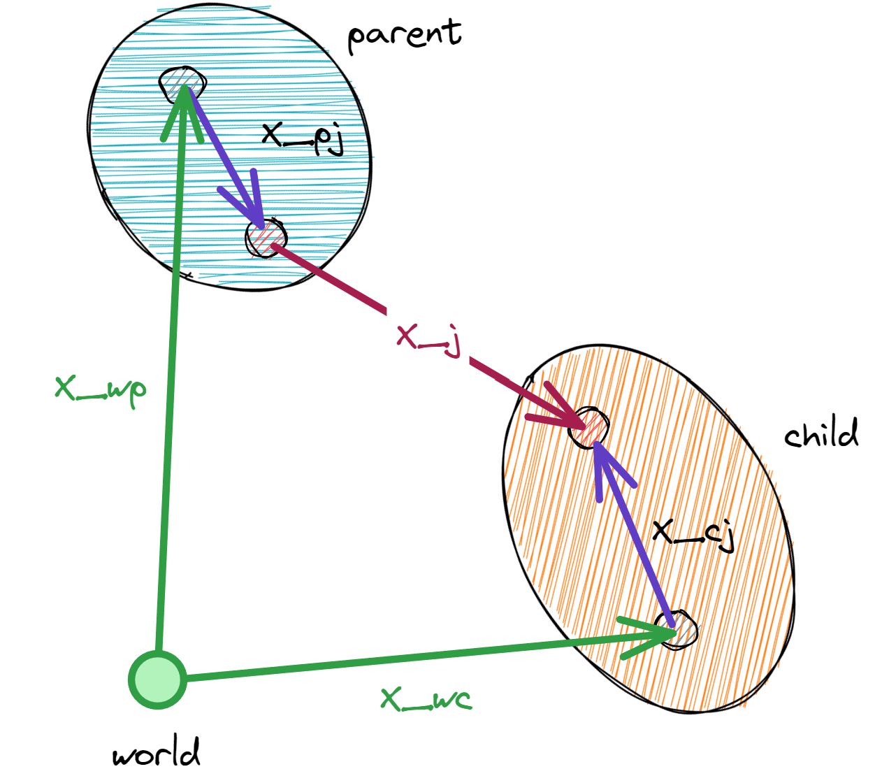
Articulated rigid-body mechanisms are kinematically described by the joints that connect the bodies as well as the relative transform from the parent and child body to the respective anchor frames of the joint in the parent and child body:
Symbol |
Description |
|---|---|
x_wp |
World transform of the parent body (stored at |
x_wc |
World transform of the child body (stored at |
x_pj |
Transform from the parent body to the joint parent anchor frame (defined by |
x_cj |
Transform from the child body to the joint child anchor frame (defined by |
x_j |
Joint transform from the joint parent anchor frame to the joint child anchor frame |
In the forward kinematics, the joint transform is determined by the joint coordinates (generalized joint positions State.joint_q and velocities State.joint_qd).
Given the parent body’s world transform \(x_{wp}\) and the joint transform \(x_{j}\), the child body’s world transform \(x_{wc}\) is computed as:
Newton’s public newton.eval_fk() writes State.body_qd using that
COM/world convention, and newton.eval_ik() expects the same convention
when recovering generalized state from maximal body state. For FREE and
DISTANCE joints, the
recovered generalized velocities are rotated back into the joint parent frame.
- newton.eval_fk(model, joint_q, joint_qd, state, mask=None, indices=None, body_flag_filter=BodyFlags.ALL)[source]
Evaluates the model’s forward kinematics given the joint coordinates and updates the state’s body information (
State.body_qandState.body_qd).The written
State.body_qdvalues use Newton’s public body-twist convention(v_com_world, omega_world).Note
CABLEbody transforms are not changed bynewton.eval_fk(); they are advanced directly bynewton.solvers.SolverVBD.- Parameters:
model (Model) – The model to evaluate.
joint_q (wp.array[float]) – Generalized joint position coordinates, shape [joint_coord_count], float
joint_qd (wp.array[float]) – Generalized joint velocity coordinates, shape [joint_dof_count], float
state (State | Model | object) – The state-like target to update (e.g.,
StateorModel).mask (wp.array[bool] | None) – The mask to use to enable / disable FK for an articulation. If None then treat all as enabled, shape [articulation_count], bool
indices (wp.array[int] | None) – Integer indices of articulations to update. If None, updates all articulations. Cannot be used together with mask parameter.
body_flag_filter (int) – Body flag filter controlling which bodies are written to in
state.body_qandstate.body_qd. Default updates both dynamic and kinematic bodies. Bodies that do not match the filter retain their existing values; they are not zeroed or invalidated.
- newton.eval_ik(model, state, joint_q, joint_qd, mask=None, indices=None, body_flag_filter=BodyFlags.ALL)[source]
Evaluates the model’s inverse kinematics given the state’s body information (
State.body_qandState.body_qd) and updates the generalized joint coordinates joint_q and joint_qd.The input
State.body_qdis interpreted using Newton’s public body-twist convention(v_com_world, omega_world). For FREE and DISTANCE joints, the recoveredjoint_qdlinear entries are referenced at the child COM and expressed in the joint parent frame.- Parameters:
model (Model) – The model to evaluate.
state (State | Model | object) – The state-like object with the body’s maximal coordinates (positions
State.body_qand velocitiesState.body_qd) to use.joint_q (wp.array[float]) – Generalized joint position coordinates, shape [joint_coord_count], float
joint_qd (wp.array[float]) – Generalized joint velocity coordinates, shape [joint_dof_count], float
mask (wp.array[bool] | None) – Boolean mask indicating which articulations to update. If None, updates all (or those specified by indices).
indices (wp.array[int] | None) – Integer indices of articulations to update. If None, updates all articulations.
body_flag_filter (int) – Body flag filter controlling which joints are written based on each joint’s child body flag. Default updates joints for both dynamic and kinematic child bodies. Entries that do not match the filter retain their existing values in
joint_qandjoint_qd.
Note
The mask and indices parameters are mutually exclusive. If both are provided, a ValueError is raised.
Orphan joints#
An orphan joint is a joint that is not part of any articulation and whose child body is not reachable through any articulated joint (i.e. the child has no articulated path back to the rest of the model). This situation can arise when:
The USD asset does not define a
PhysicsArticulationRootAPIon any prim, so no articulations are discovered during parsing.A joint connects two bodies that are not under any
PhysicsArticulationRootAPIprim, even though other articulations exist in the scene.
A joint that is excluded from every add_articulation() call but whose two bodies are already reachable through the articulation tree is not an orphan joint; it is a loop-closing joint (see Loop closure) and is handled separately.
When orphan joints are detected during USD parsing (add_usd()), Newton issues a warning that lists the affected joint paths.
Validation and finalization
By default, finalize() raises a ValueError if any orphan joint is found. (Loop-closing joints pass this check — see Loop closure.) To proceed with orphan joints, skip this validation:
model = builder.finalize(skip_validation_joints=True)
Solver compatibility
Only maximal-coordinate solvers (SolverXPBD, SolverSemiImplicit) support orphan joints.
Generalized-coordinate solvers (SolverFeatherstone, SolverMuJoCo) require every joint to belong to an articulation.
(Loop-closing joints are not orphan joints and are handled separately — see Loop closure.)
Loop closure#
Newton’s add_joint_*() methods author kinematic
trees: each body has at most one parent joint, so the joints alone cannot
form a closed kinematic loop (for example a four-bar linkage or a parallel
mechanism). Closed loops must instead be expressed by declaring the topology
as a tree and adding a separate joint that re-couples the open end.
To close a loop, create the loop-closing joint with
add_joint_*() but omit it from the
``joint_list`` passed to add_articulation(),
so the articulation graph remains a tree. The omitted joint is a
loop-closing joint: its two bodies are both already reachable through
the tree, which distinguishes it from an
orphan joint (whose child has no articulated path
and which finalize() rejects unless
skip_validation_joints=True).
builder = newton.ModelBuilder()

# Fixed root attached to the world.
root = builder.add_link()
builder.add_shape_box(root, hx=0.1, hy=0.1, hz=0.1)
j_root = builder.add_joint_fixed(parent=-1, child=root)

# Child A: revolute about Z, hinged on the root at +X.
child_a = builder.add_link()
builder.add_shape_box(child_a, hx=0.5, hy=0.05, hz=0.05)
j_a = builder.add_joint_revolute(
    parent=root,
    child=child_a,
    axis=newton.Axis.Z,
    parent_xform=wp.transform(wp.vec3(1.0, 0.0, 0.0), wp.quat_identity()),
)

# Child B: revolute about Z, hinged on the root at -X.
child_b = builder.add_link()
builder.add_shape_box(child_b, hx=0.5, hy=0.05, hz=0.05)
j_b = builder.add_joint_revolute(
    parent=root,
    child=child_b,
    axis=newton.Axis.Z,
    parent_xform=wp.transform(wp.vec3(-1.0, 0.0, 0.0), wp.quat_identity()),
)

# Loop-closing joint: a fixed joint between the two children. Authored with
# add_joint_* exactly like a tree joint, but deliberately left out of the
# articulation below.
j_loop = builder.add_joint_fixed(parent=child_a, child=child_b)

# Only the tree joints (j_root, j_a, j_b) go into the articulation;
# j_loop is excluded so the articulation graph remains a tree.
builder.add_articulation([j_root, j_a, j_b])

model = builder.finalize()
Importing from USD. The same omit-from-articulation pattern is the
standard way UsdPhysics expresses loop closures, and Newton’s USD importer
honors it. Set the physics:excludeFromArticulation attribute to true
on a PhysicsJoint prim, and add_usd() will
register the joint with the builder via the normal add_joint_* path but
leave it out of the surrounding add_articulation()
call — producing exactly the topology shown above. This is how
a USD asset can author a four-bar linkage or other parallel mechanism.
Note
A loop-closing joint passes finalize()
validation by default — because its two bodies are already reachable
through the tree, the orphan-joint check does not fire and
skip_validation_joints=True is not required. Each solver then
handles the loop-closing joint differently:
Maximal-coordinate solvers track state as per-body transforms (
body_q/body_qd) and enforce joints as pairwise body constraints, so the loop-closure joint is solved alongside the tree joints with no special-casing. UnderSolverXPBDandSolverSemiImplicit,j_loopkeeps its full joint behavior — drive (joint_target_ke/joint_target_kd,control.joint_f) and joint limits are applied alongside the loop-closure constraint, subject to each solver’s general joint-feature support (see Joint Feature Support).SolverVBDandSolverKaminouse the same flat per-joint iteration but support a narrower set of joint types and features, so the same loop-closure pattern works only within their respective supported subsets.Generalized-coordinate solvers carry only tree-joint coordinates in their state vector and must handle the loop closure separately.
SolverMuJoCoenforces each loop-closure joint as a bilateral coupling at compile time, which restricts the supported joint types and drops joint-level features (see the note below).SolverFeatherstonehas no such synthesis path: the loop-closure joint contributes no DOFs and the loop closure is silently not enforced.
In all cases the loop-closing joint is invisible to newton.eval_fk(),
newton.eval_ik(), and ArticulationView —
those walk the articulation tree only.
Note
SolverMuJoCo supports only a subset of joint
types as loop closures, and the loop-closing joint loses its joint-level
features (drive, limits, armature, friction). See
Loop closures for the supported types and MuJoCo-specific
behavior.